Creating Shapes#
The Polygon Object#
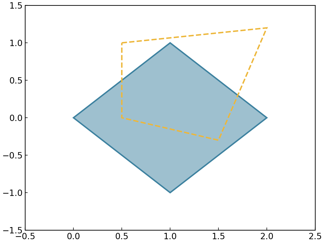
GraphingLib allows you to create polygons by specifying their vertices. Here is an example with a random shape:
polygon1 = gl.Polygon(
    vertices=[(0, 0), (1, 1), (2, 0), (1, -1)],
    edge_color="C0",
    line_width=2,
    line_style="solid",
    fill=True,
    fill_color="C0",
    fill_alpha=0.5,
)

polygon2 = gl.Polygon(
    vertices=[(0.5, 1), (2, 1.2), (1.5, -0.3), (0.5, 0)],
    edge_color="C1",
    line_width=2,
    line_style="dashed",
    fill=False,
)

fig = gl.Figure(x_lim=(-0.5, 2.5), y_lim=(-1.5, 1.5))
fig.add_elements(polygon1, polygon2)
fig.show()

The only required parameter is vertices, but you can customize the appearance of the polygon by specifying the other parameters above. The real power of the Polygon object comes from its methods. Here are some methods used to get information about a polygon:
print(polygon1.area) # 2.0
print(polygon1.perimeter) # about 5.66
print(polygon1.get_centroid_coordinates()) # (1.0, 0.0)
# Check if a point is inside the polygon
print(gl.Point(1, 0) in polygon1) # True
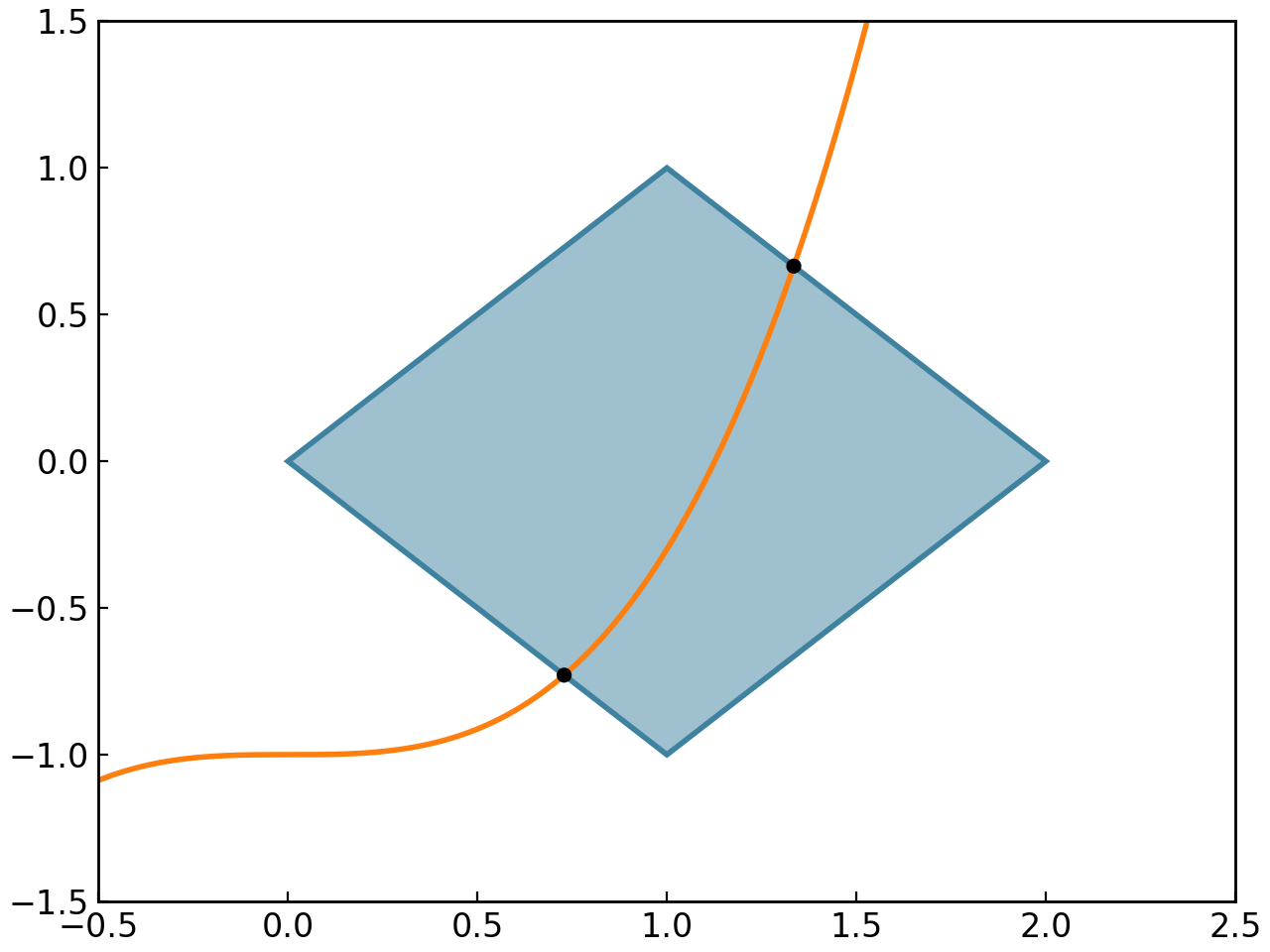
# Get the intersection points of the polygon with a curve, or the intersection points of the edges of two polygons
curve = gl.Curve.from_function(lambda x: 0.7 * x**3 - 1, x_min=-1, x_max=3, color="C1")
points = polygon1.create_intersection_points(curve)
fig = gl.Figure(x_lim=(-0.5, 2.5), y_lim=(-1.5, 1.5))
fig.add_elements(polygon1, curve, *points)
fig.show()

With GraphingLib, whenever you see a get_..._coordinates method, you can safely assume there also exists a create_..._point or create_..._points method in order to get Point objects instead of coordinates (and vice versa).
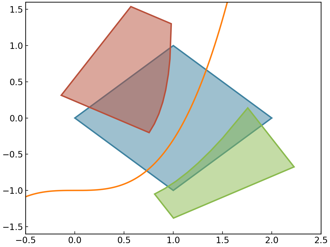
There are also many methods which manipulate and transform polygons. Here are some examples of splitting, translating, and rotating polygons:
# Split a polygon into two using a Curve
split_left, split_right = polygon1.split(curve)
split_left.fill_color = "C2"
split_left.edge_color = "C2"
split_right.fill_color = "C3"
split_right.edge_color = "C3"

# Translate and rotate the split polygons
split_left.translate(-0.2, 0.5)
split_left.rotate(15)
split_right.translate(0.2, -0.5)
split_right.rotate(-15)

fig = gl.Figure(x_lim=(-0.5, 2.5), y_lim=(-1.6, 1.6))
fig.add_elements(polygon1, curve, split_left, split_right)
fig.show()

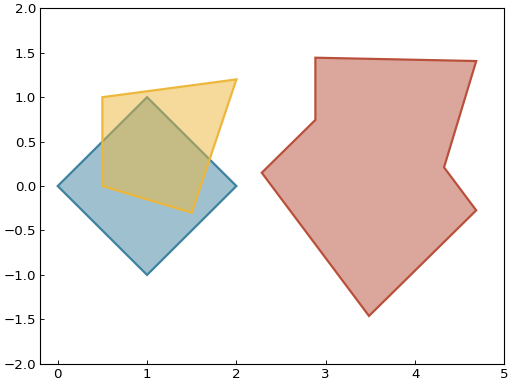
And here are some examples of unions, scaling and skewing:
polygon2.fill = True
polygon2.fill_color = "C1"
polygon2.line_style = "solid"

# Create the union of two polygons
union = polygon1.create_union(polygon2)
union.fill_color = "C2"
union.edge_color = "C2"

# Scale, skew, and apply arbitrary linear transformation to the union
union.scale(x_scale=1.2, y_scale=1.4)
union.skew(0, -10)
union.translate(2.5, 0)

fig = gl.Figure(x_lim=(-0.2, 5), y_lim=(-2, 2))
fig.add_elements(polygon1, polygon2, union)
fig.show()

Some of the most common shapes, such as rectangles and circles, have their dedicated classes to simplify their creation. These classes are detailed below.
The Rectangle Object#
Rectangles can be created easily by creating an instance of the Rectangle class as shown below:
# Create a Rectangle from the bottom left corner
rect = gl.Rectangle(x_bottom_left=0, y_bottom_left=0, width=10, height=10)

# Create a Rectangle from its center
rect2 = gl.Rectangle.from_center(x=0, y=0, width=10, height=10)
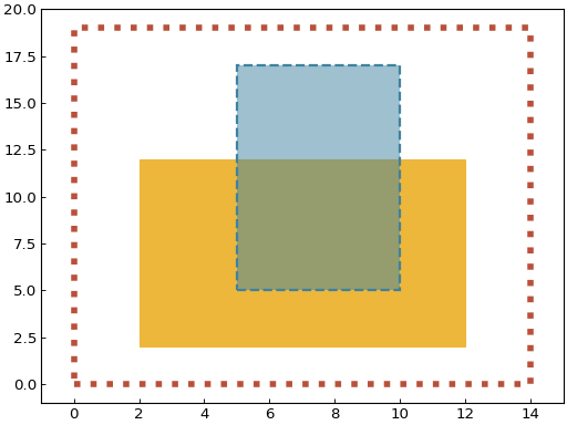
You can customize the appearance of Rectangles by specifying the following optional parameters: edge_color, line_width, line_style, fill (True or False), fill_color, and fill_alpha. Here is an example with different styles of Rectangles:
rect1 = gl.Rectangle(
    x_bottom_left=2,
    y_bottom_left=2,
    width=10,
    height=10,
    fill_color="C1",
    edge_color="C1",
    line_width=1,
    line_style="solid",
    fill=True,
    fill_alpha=1,
)

rect2 = gl.Rectangle(
    x_bottom_left=5,
    y_bottom_left=5,
    width=5,
    height=12,
    fill_color="C0",
    edge_color="C0",
    line_width=2,
    line_style="dashed",
    fill=True,
    fill_alpha=0.5,
)

rect3 = gl.Rectangle(
    x_bottom_left=0,
    y_bottom_left=0,
    width=14,
    height=19,
    edge_color="C2",
    line_width=5,
    line_style="dotted",
    fill=False,
)

figure = gl.Figure(x_lim=(-1, 15),y_lim=(-1, 20))
figure.add_elements(rect1, rect2, rect3)
figure.show()
All Polygon methods can also be used with Rectangle objects.
The Circle Object#
GraphingLib also lets you plot Circles. You can create a Circle by specifying its center point and radius:
circle = gl.Circle(x_center=0, y_center=0, radius=10)
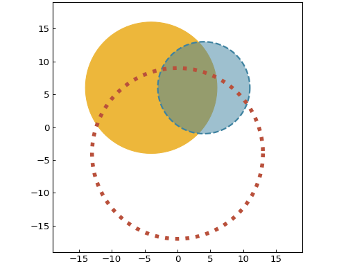
You can customize the appearance of Circles by specifying the following optional parameters: color, line_width, line_style, fill (True or False), and fill_alpha. Here is an example with different styles of Circles:
circle1 = gl.Circle(
    x_center=-4,
    y_center=6,
    radius=10,
    fill_color="C1",
    edge_color="C1",
    line_width=1,
    line_style="solid",
    fill=True,
    fill_alpha=1,
)

circle2 = gl.Circle(
    x_center=4,
    y_center=6,
    radius=7,
    fill_color="C0",
    edge_color="C0",
    line_width=2,
    line_style="dashed",
    fill=True,
    fill_alpha=0.5,
)

circle3 = gl.Circle(
    x_center=0,
    y_center=-4,
    radius=13,
    fill_color="C2",
    edge_color="C2",
    line_width=5,
    line_style="dotted",
    fill=False,
)

# Aspect ratio set to 1 to make the circles look round
figure = gl.Figure(x_lim=(-19, 19), y_lim=(-19, 19), aspect_ratio=1)
figure.add_elements(circle1, circle2, circle3)
figure.show()

As with Rectangles, all Polygon methods can also be used with Circle objects.
Since Circle objects actually inherit from Polygon, they aren’t perfectly round, and so area and perimeter calculations are approximations. You can get arbitrarily close to the true values by increasing the number of points used to approximate the circle. This can be done by setting the number_of_points parameter when creating the Circle object. The default value is 100, which gives you 99.9% accuracy for the area and even better for the perimeter. Here is an example:
circle = gl.Circle(x_center=0, y_center=0, radius=10, number_of_points=1000)
print(circle.area)
print(circle.perimeter)
The Ellipse Object#
The Ellipse class is similar to Circle, but allows you to specify different radii for the x and y axes. You can also apply a rotation angle to the ellipse. Create an Ellipse by specifying its center point, x radius, and y radius:
ellipse = gl.Ellipse(x_center=0, y_center=0, x_radius=10, y_radius=5)
The key differences between Ellipse and Circle are:
Two independent radii: Use
x_radiusandy_radiusinstead of a singleradiusparameterOptional rotation: You can rotate the ellipse using the
angleparameter (in degrees)Width and height properties: Access or set dimensions via
width(2 × x_radius) andheight(2 × y_radius)
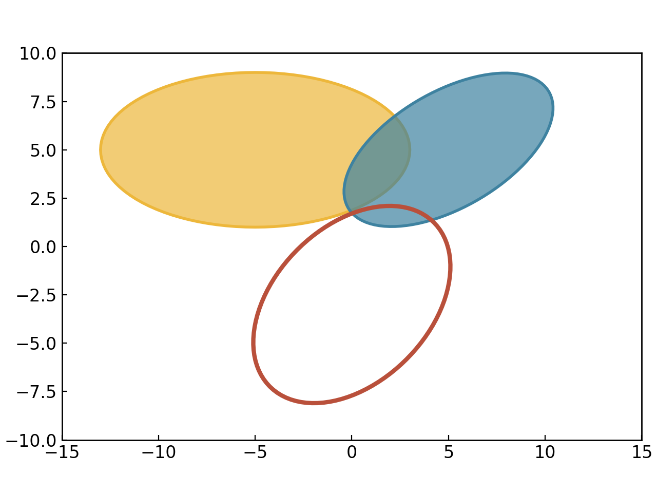
Here is an example with different ellipses:
ellipse1 = gl.Ellipse(
    x_center=-5,
    y_center=5,
    x_radius=8,
    y_radius=4,
    fill_color="C1",
    edge_color="C1",
    line_width=2,
    fill=True,
    fill_alpha=0.7,
)

ellipse2 = gl.Ellipse(
    x_center=5,
    y_center=5,
    x_radius=6,
    y_radius=3,
    fill_color="C0",
    edge_color="C0",
    line_width=2,
    fill=True,
    fill_alpha=0.7,
    angle=30,  # Rotated by 30 degrees
)

ellipse3 = gl.Ellipse(
    x_center=0,
    y_center=-3,
    x_radius=6,
    y_radius=4,
    edge_color="C2",
    line_width=3,
    fill=False,
    angle=45,
)

figure = gl.Figure(x_lim=(-15, 15), y_lim=(-10, 10), aspect_ratio=1)
figure.add_elements(ellipse1, ellipse2, ellipse3)
figure.show()

Like Circles, Ellipse objects inherit from Polygon and use point approximation, so circumference and area calculations are approximations. The number_of_points parameter can be adjusted for better accuracy.
The Arrow Object#
GraphingLib also lets you plot Arrows. You can create an Arrow by specifying its start and end points:
arrow = gl.Arrow(pointA=(0, 0), pointB=(10, 10))
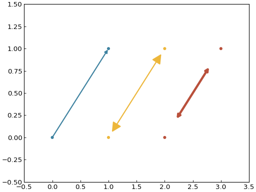
You can customize the appearance of Arrows by specifying the following optional parameters: color, width (the line width), head_size, two_sided (True or False), and shrink. The shrink parameter is a float between 0 and 0.5 which shortens the arrow from both ends by the given percentage (0 doesn’t shrink at all, 0.5 makes the arrow disappear completely). Here is an example with different styles of Arrows:
arrow1 = gl.Arrow(
    pointA=(0, 0),
    pointB=(1, 1),
    color="C0",
    shrink=0,  # default, no shrinking
)
arrow2 = gl.Arrow(
    pointA=(1, 0),
    pointB=(2, 1),
    color="C1",
    shrink=0.05,
    two_sided=True,
    head_size=3,
)
arrow3 = gl.Arrow(
    pointA=(2, 0),
    pointB=(3, 1),
    color="C2",
    shrink=0.2,
    two_sided=True,
    width=4,
)

# Create points at the start and end of the arrows (to illustrate the shrinking)
point1 = gl.Point(0, 0, face_color="C0")
point2 = gl.Point(1, 0, face_color="C1")
point3 = gl.Point(2, 0, face_color="C2")
point4 = gl.Point(1, 1, face_color="C0")
point5 = gl.Point(2, 1, face_color="C1")
point6 = gl.Point(3, 1, face_color="C2")

fig = gl.Figure(y_lim=(-0.5, 1.5), x_lim=(-0.5, 3.5))
fig.add_elements(arrow1, arrow2, arrow3)
fig.add_elements(point1, point2, point3)
fig.add_elements(point4, point5, point6)
fig.show()

The Line object#
It is possible to add lines to figures. Similarly to the Arrow object, simply specify the two end points
line = gl.Line((0, 0), (1, 1))
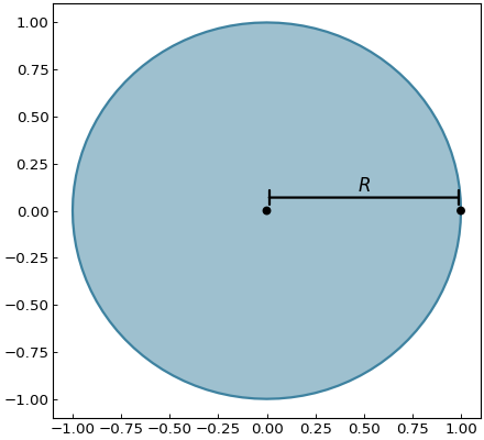
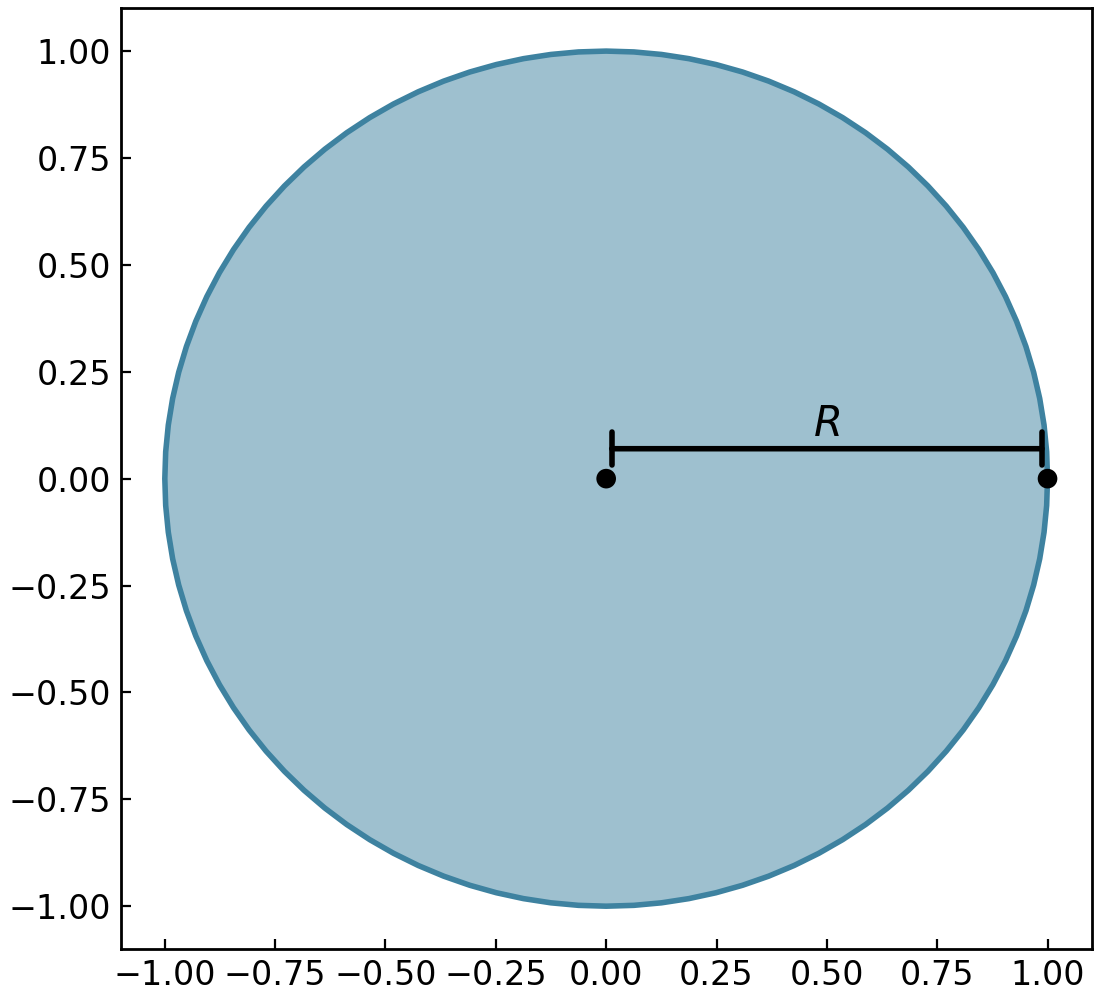
It is possible to change the width of the line with the width parameter. The capped_line parameter allows you to add perpendicular caps to both ends of the line. The width of those caps can be controlled with the cap_width parameter
# Creating a circle and finding a point at 45 degrees on the circumference
circle = gl.Circle(0, 0, 1, line_width=2, edge_color="C0", fill_color="C0")
center = gl.Point(0, 0, marker_size=50)
point = gl.Point(1, 0, marker_size=50)

# Adding a line to display the radius of the circle
line = gl.Line(
    (0, 0.07), (point.x, point.y + 0.07), capped_line=True, cap_width=1
)
text = gl.Text(0.5, 0.1, r"$R$", font_size=15)

# Display the elements
fig = gl.Figure(size=(5.5, 5))
fig.add_elements(circle, point, line, center, text)
fig.show()