Creating a simple figure with the SmartFigure#
Quickstart#
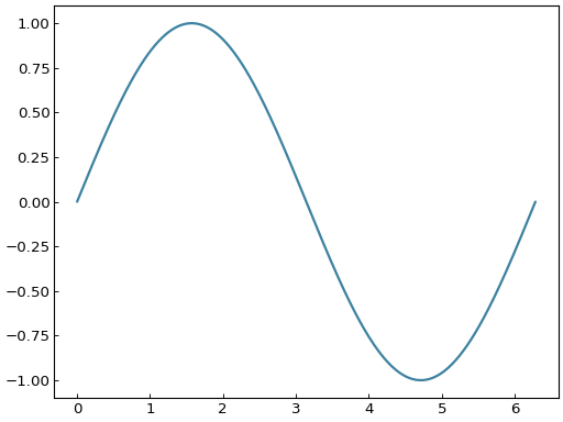
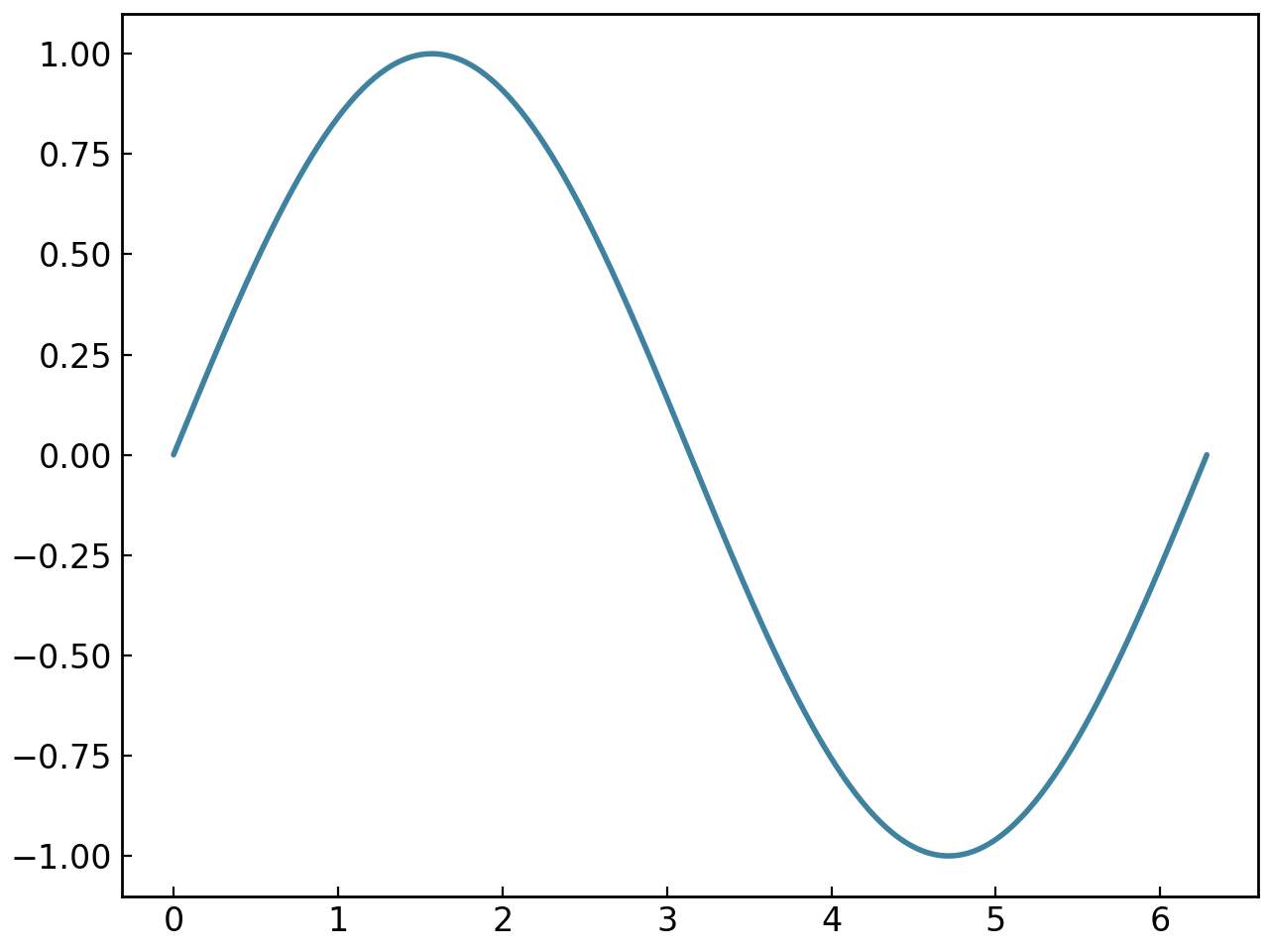
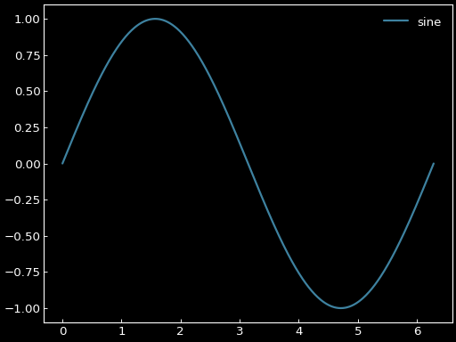
Creating a basic figure using the SmartFigure object is easy. The example below shows how to create a sine curve and display it.
sine = gl.Curve.from_function(lambda x: np.sin(x), 0, 2 * np.pi)

figure = gl.SmartFigure(elements=sine)
figure.show()

The show() method is used to show the figure on screen. It is also possible to use the save() method to save the figure to a specified path while setting certain options like the resolution (dpi).
See also
For the documentation on the from_function() method, see the handbook section on curves.
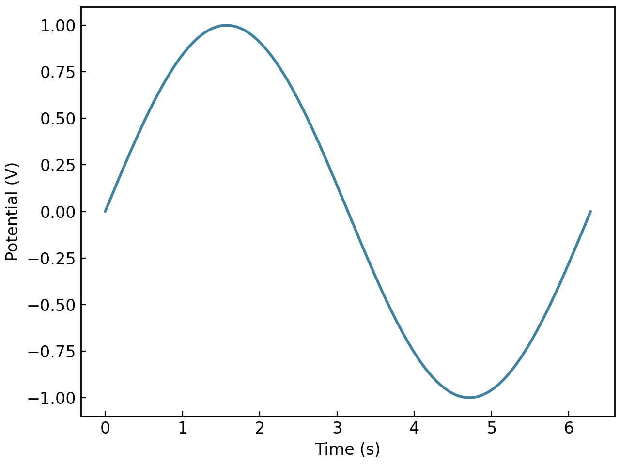
We can specify the axis labels by using the x_label and y_label parameters of the SmartFigure.
figure = gl.SmartFigure(x_label="Time (s)", y_label="Potential (V)", elements=sine)
figure.show()

As a general note, all parameters available in the constructor are also available as properties. This means that you can set or modify them after creating the SmartFigure. For further informations on the available parameters and methods, please refer to the handbook section on complex SmartFigures or the reference section on SmartFigure objects.
Creating multi-subplot layouts#
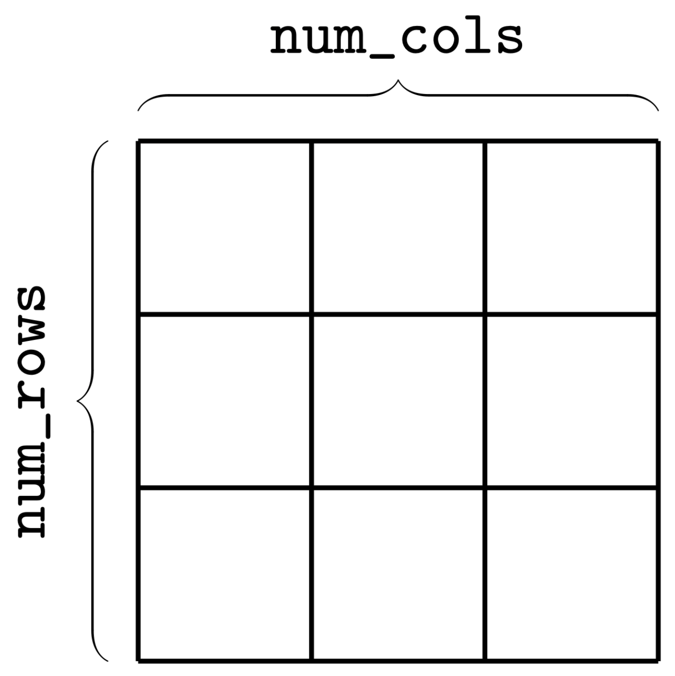
To create a figure with a grid of subplots, the dimensions of the canvas first need to be defined using the num_rows and num_cols parameters, shown in the figure below. This grid is then used to place each child plot in the SmartFigure.
If you already have a SmartFigure being used as a single plot and want to turn it into a layout, first increase num_rows or num_cols. This keeps the original plot as the child plot in the top-left position of the new layout.
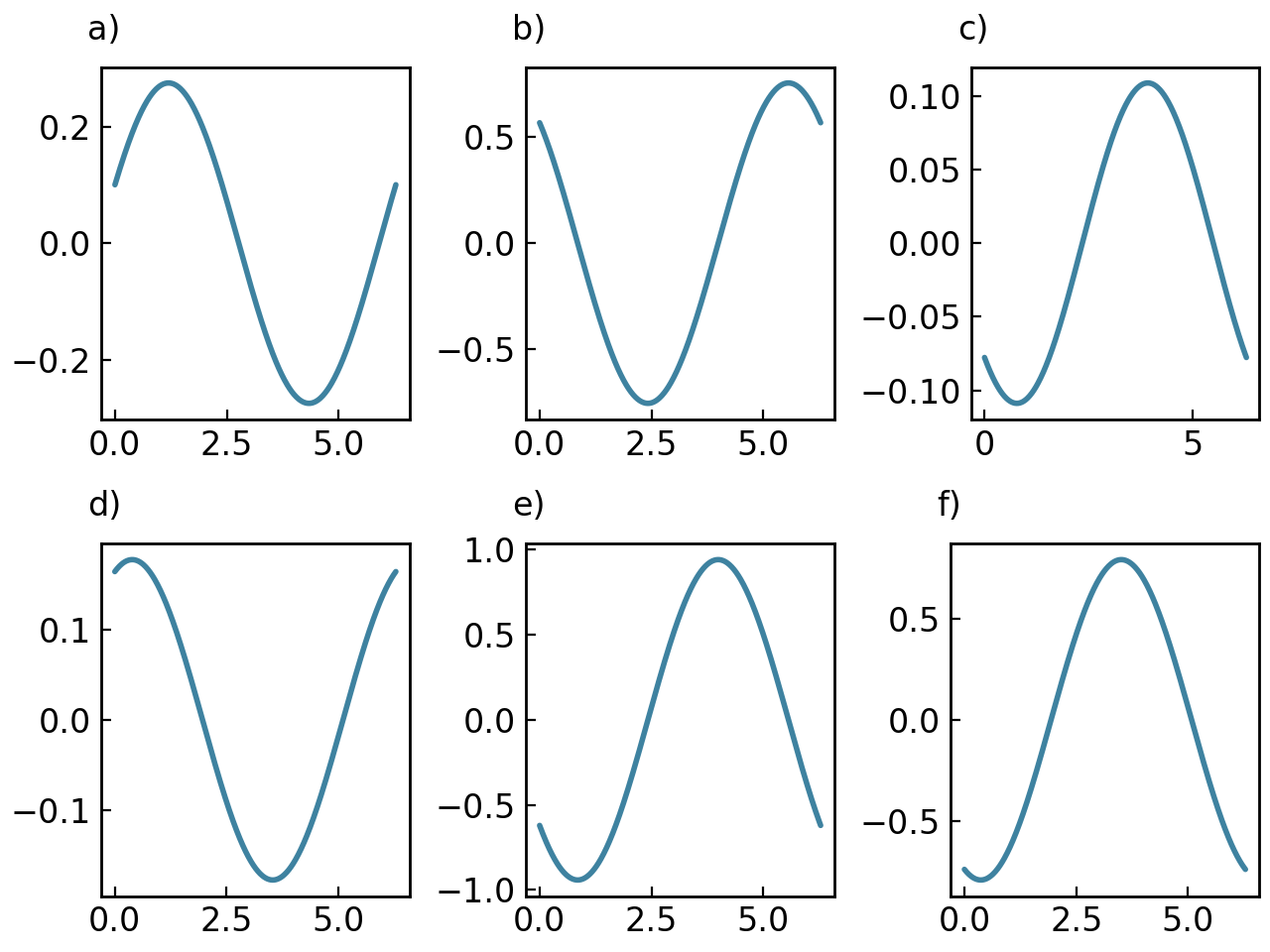
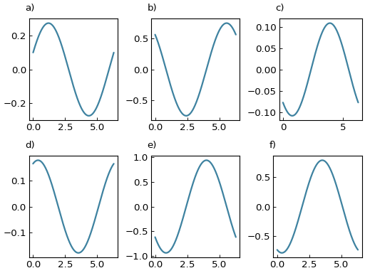
For example, let’s create a SmartFigure with 2 rows, 3 columns and 6 random curves:
random_curve = lambda: gl.Curve.from_function(
    lambda x: np.random.rand() * np.sin(x + np.random.rand() * 2 * np.pi), 0, 2*np.pi
)
figure = gl.SmartFigure(2, 3, elements=[random_curve() for _ in range(6)])
figure.show()
In this example, the elements list fills the grid from left to right, then top to bottom. Each occupied position becomes its own child plot.
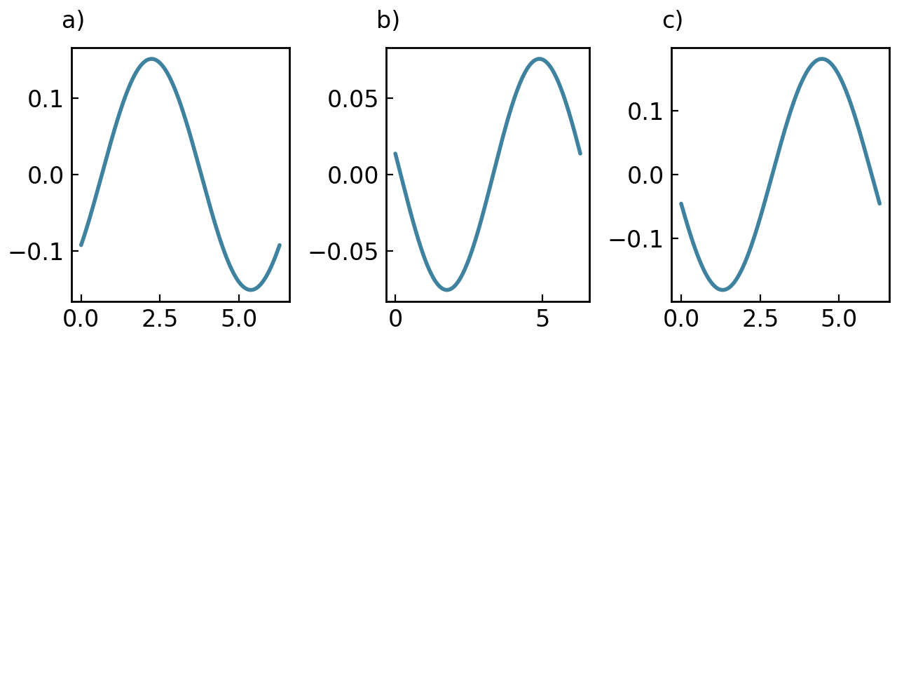
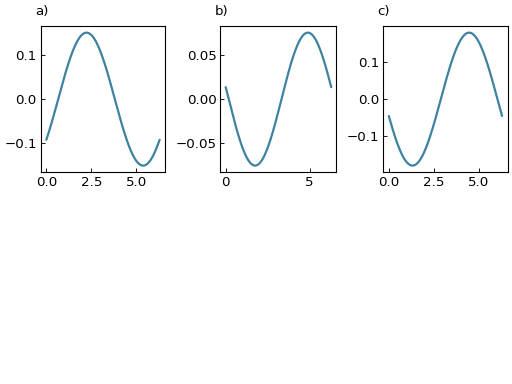
It is also possible to add elements to a preexisting figure using the add_elements() method:
figure = gl.SmartFigure(2, 3)
figure.add_elements(*[random_curve() for _ in range(3)])  # Fills the first three positions
figure.show()
When used on a layout, add_elements() walks through the grid from left to right, then top to bottom. If a child plot already exists in a position, the new element is added to it. If the position is empty, a new child plot is created there.
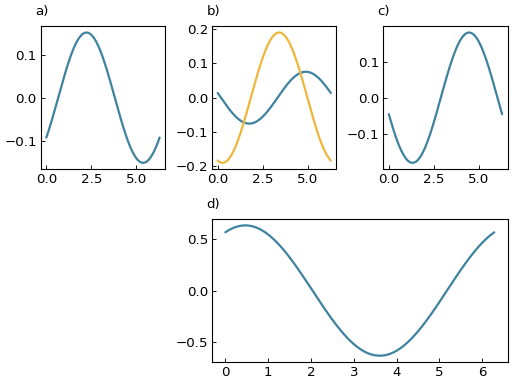
The __setitem__() method can also be used to fill specific positions in the layout by specifying their position in the grid, exactly how two-dimensional numpy arrays are indexed. Assigning a Plottable to a cell creates a child plot there. Attributing None to a position removes the child plot occupying it. Slicing is also supported to add elements to or remove elements from multiple rows or columns at once. Here are some examples:
# Remove the elements from the bottom row
figure[1, 0] = None
figure[1, 1] = None
figure[1, 2] = None

# Add a curve that spans the last two subplots of the bottom row
figure[1, 1:] = random_curve()

# Add a curve to the second child plot
figure[0, 1] += random_curve()

figure.show()

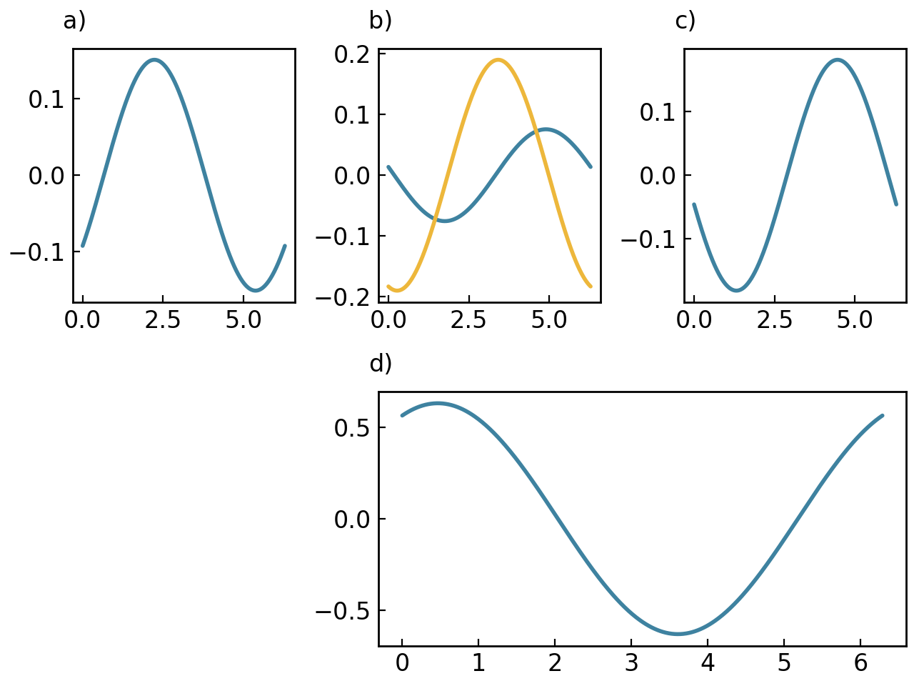
The object returned by indexing is itself a SmartFigure, which means you can work on that child plot directly:
child_plot = figure[0, 1]
child_plot += random_curve()
figure.show()
Tip
When an element spans multiple cells, you can access, modify, or remove it by clicking on any cell it occupies. For example, to remove the curve that spans [1, 1:], you can use figure[1, 1] = None or figure[1, 2] = None. See the Advanced SmartFigure Usage and Complete Reference section for more details on multi-cell element access.
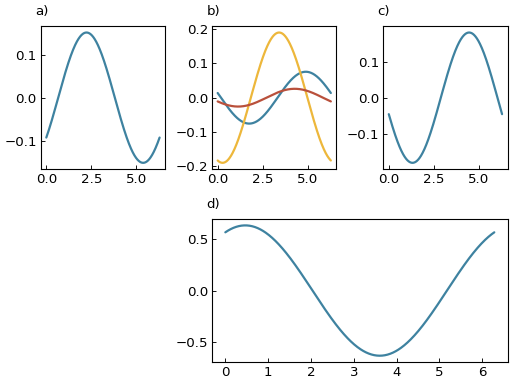
The advantage of the SmartFigure class is that you can also insert an existing SmartFigure inside another one:
# Insert the previous figure as a nested child in the bottom-right area
figure[1, 1:] = figure.copy()
figure.show()

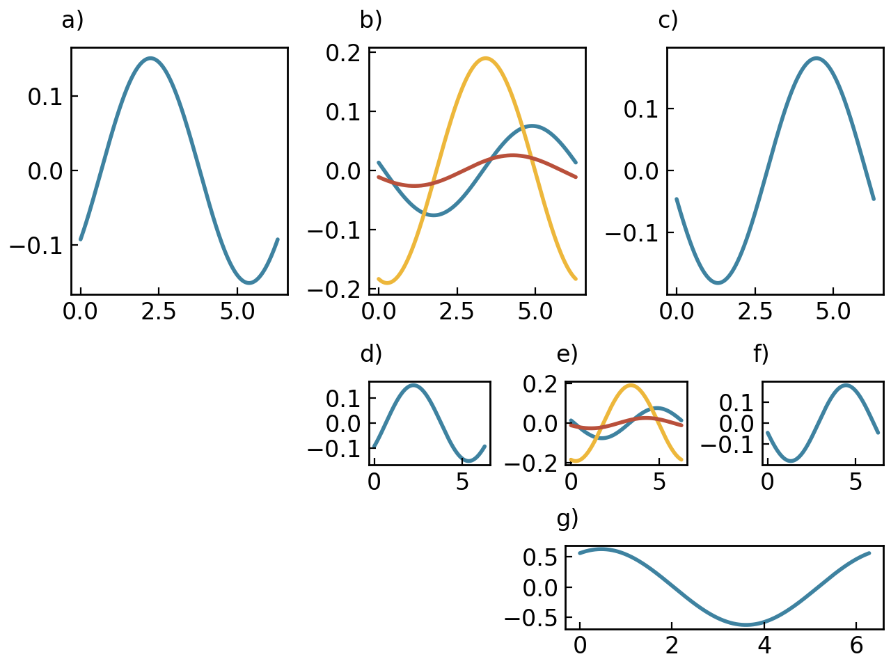
Assigning plottables to cells creates child plots controlled by the parent layout. Inserting an existing SmartFigure creates a nested figure that keeps its own labels, title, styles, legend behavior, and other subplot-level settings. This means that complex figures with different sets of parameters per area can be created by nesting SmartFigure objects.
In the previous examples, there were labels a), b), c), … at the top left corner of each subplot. These labels are refered to as reference labels and are useful to identify each subplot when inserting the figure in a document. The boolean parameter reference_labels (in the SmartFigure constructor or as a property) can turn these on or off.
Legends in SmartFigures#
Legends in SmartFigures can be toggled with the show_legend parameter which applies to all plots drawn directly in the SmartFigure. Explicitly nested SmartFigure objects still control their own legends independently. The legends in a SmartFigure can be added separately for every child plot or as a single legend combining the labels of every plot. This option is controlled by the general_legend parameter. By default, it is set to False so that each subfigure controls its own legend. The two images below illustrate the different legend options. Note that it is also possible to control the position of the legend using the legend_loc parameter.
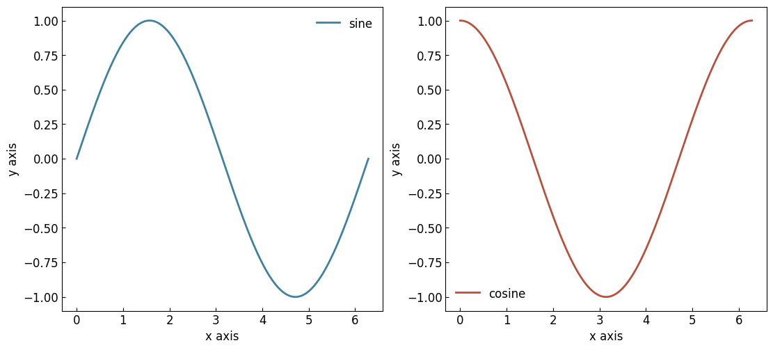
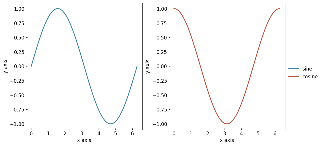
Figure styles#
The figure_style parameter of the SmartFigure class allows you to specify a predefined style to use to change the appearance of the figure and the elements plotted inside it. You can specify a predefined style as follows:
figure = gl.SmartFigure(x_label="Time (s)", y_label="Potential (V)", figure_style="plain")
There are 3 categories of predefined styles.
GraphingLib styles are styles that we have created and that are always available. The default style called “plain” is one of these, and you can see the others here.
All Matplotlib styles are also available. You can see the list of available Matplotlib styles here. To use the default Matplotlib style, simply specify
"matplotlib"as the style.You can also create, save and specify your own custom styles, and you can even set your preferred style as the default style.
It is important to note that the parameters controlled by the specified style can be overridden simply by specifying the desired options. The explicitly specified options will always be prioritized.
See also
For the instructions on how to write your own figure style file and see what parameters are controlled by the figure style files, see Writing your own figure style file.
Style customization#
Besides the figure_style parameter, it is possible to further customize a figure’s appearance by using the set_visual_params() or the set_rc_params() methods. The first method allows you to specify the options directly, while the second method allows you to specify the options using a dictionary of matplotlib rc parameters. Only the most common options are available using the first method, while the second method allows you to give any matplotlib rc parameter. Here is an example using the first method:
figure = gl.SmartFigure(x_label="Time (s)", y_label="Potential (V)", figure_style="plain")
figure.set_visual_params(
    use_latex=True,
    font_size=12,
    axes_edge_color="red",
)
And here is another example for the second method:
figure = gl.SmartFigure(x_label="Time (s)", y_label="Potential (V)", figure_style="plain")
figure.set_rc_params(
    {
        "text.usetex": True,
        "font.size": 12,
        "axes.edgecolor": "red",
    }
)
Both work fine, but the first method allows to take advantage of the power of your IDE’s popup suggestions and saves the user from having to look up the matplotlib rc parameter names for the most common options.
Note
If you find yourself using the same options over and over again, you may want to create your own figure style file. It’s much easier than it sounds and will save you a lot of time! See Writing your own figure style file for more information.
Styles and customization with nested SmartFigures#
Figure style and customizations can get a bit confusing when working with nested SmartFigure objects. Here is a brief overview:
The
figure_styleparameter of the parent is applied to every nestedSmartFigurein it. Anyfigure_stylespecified in the nestedSmartFigureobjects is ignored.On the other hand, though applying style customizations to the
SmartFigureobject will apply them to every nestedSmartFigure, customizations specified in the individual nestedSmartFigureobjects are prioritized over the parentSmartFigure’s customizations. For example, this means that turning the grid on in theSmartFigurewill turn it on for every nestedSmartFigureobjects, but turning it off in an individualSmartFigurewill override the parentSmartFigure’s setting and turn it off for that nestedSmartFigureonly.
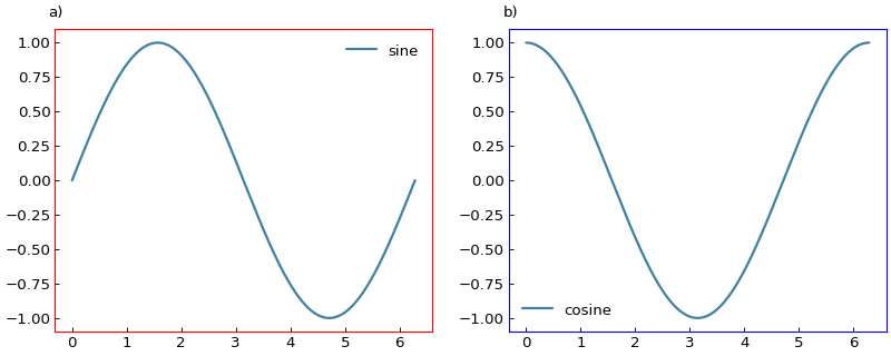
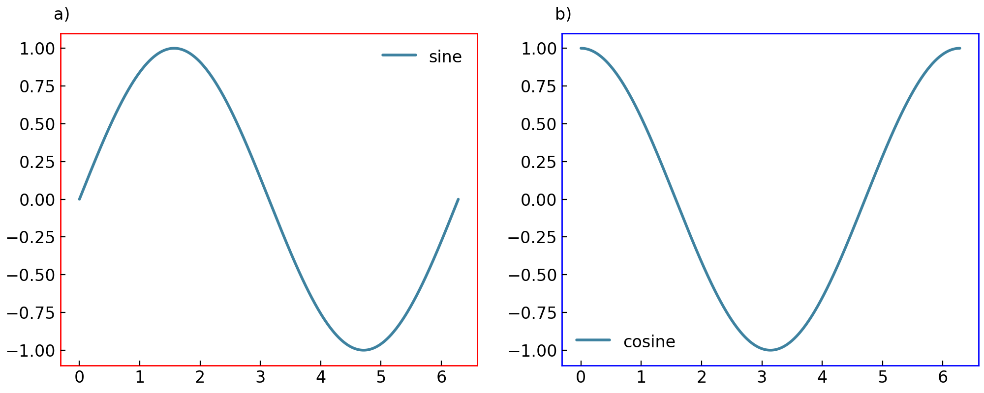
In short, the figure_style chosen in a parent SmartFigure sets a base style for the SmartFigure as a whole. Calling the set_visual_params() or the set_rc_params() methods on the SmartFigure will personalize the chosen figure_style, whereas calling these methods on the individual nested SmartFigure objects only allows them to override the parent SmartFigure’s customizations. Here is an example with customization of the axes edge colors:
# Create the curves
sine = gl.Curve.from_function(lambda x: np.sin(x), 0, 2 * np.pi, label="sine")
cosine = gl.Curve.from_function(lambda x: np.cos(x), 0, 2 * np.pi, label="cosine")

# Create the figures and add the elements
figure1 = gl.SmartFigure(figure_style="dark")
figure1.add_elements(sine)
figure2 = gl.SmartFigure(elements=cosine)

# Create the parent SmartFigure and add the figures to it
# Use the "plain" style which has a black axes edge color
parent_figure = gl.SmartFigure(num_cols=2, size=(10, 4), figure_style="plain")
parent_figure.elements = [figure1, figure2]

# Customize the axes edge color for all figures (but will be overridden for figure2)
# Note: the order of these calls does not matter,
# a nested SmartFigure will always override the parent SmartFigure
parent_figure.set_visual_params(axes_edge_color="red")
figure2.set_visual_params(axes_edge_color="blue")

# Display the parent SmartFigure
# This shows the two figures side-by-side with the "plain" style, but
# the axes edge color will be red for figure1 and blue for figure2
parent_figure.show()

# Display figure1 separately
# This shows figure1 with the "dark" style and with no axes edge color customization
figure1.show()

See Also#
Advanced SmartFigure Usage and Complete Reference - More advanced SmartFigure features
graphinglib.SmartFigure - SmartFigure API reference