Advanced SmartFigure Usage and Complete Reference

This comprehensive guide details every feature and method of the SmartFigure class. For a quick introduction to basic usage, see Creating a simple figure with the SmartFigure.

Note

As a reminder, all parameters in the SmartFigure constructor can also be set or modified later using the corresponding properties or methods.

Elements Management

The SmartFigure provides multiple ways to add and manage plot contents. Understanding the distinction between these methods is crucial for effective use, especially when switching between a single plot and a layout of child plots.

Adding Elements: All the Ways

There are four distinct ways to add elements to a SmartFigure:

1. Through the constructor with the elements parameter

2. Using the add_elements() method

3. Setting the elements property

4. Using the __setitem__() method (indexing with [])

Constructor: elements parameter

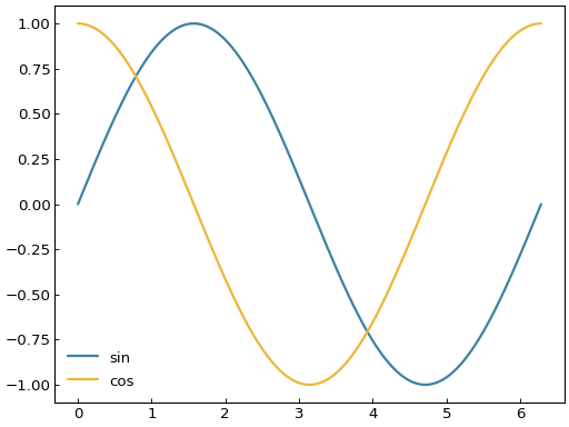
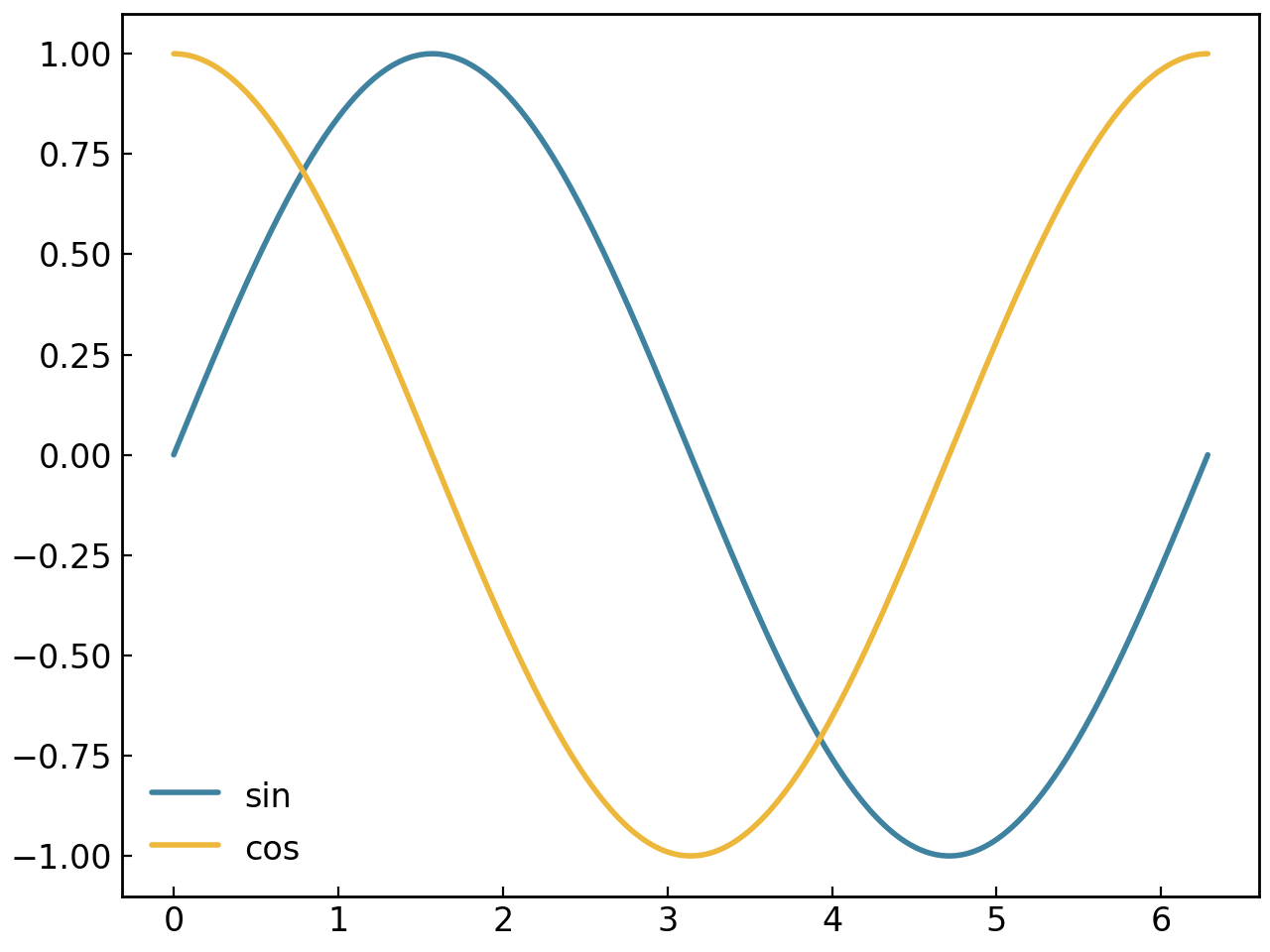
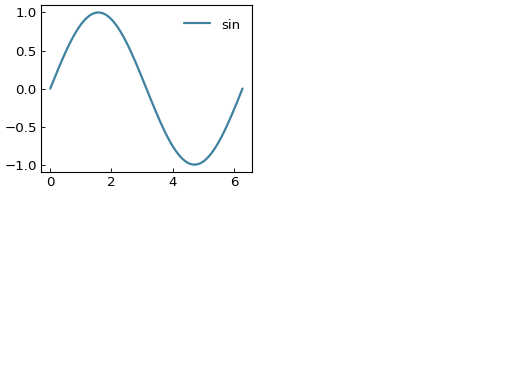
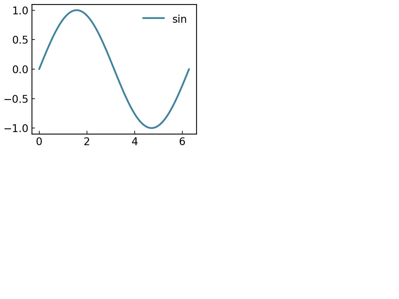
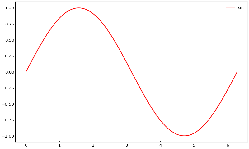
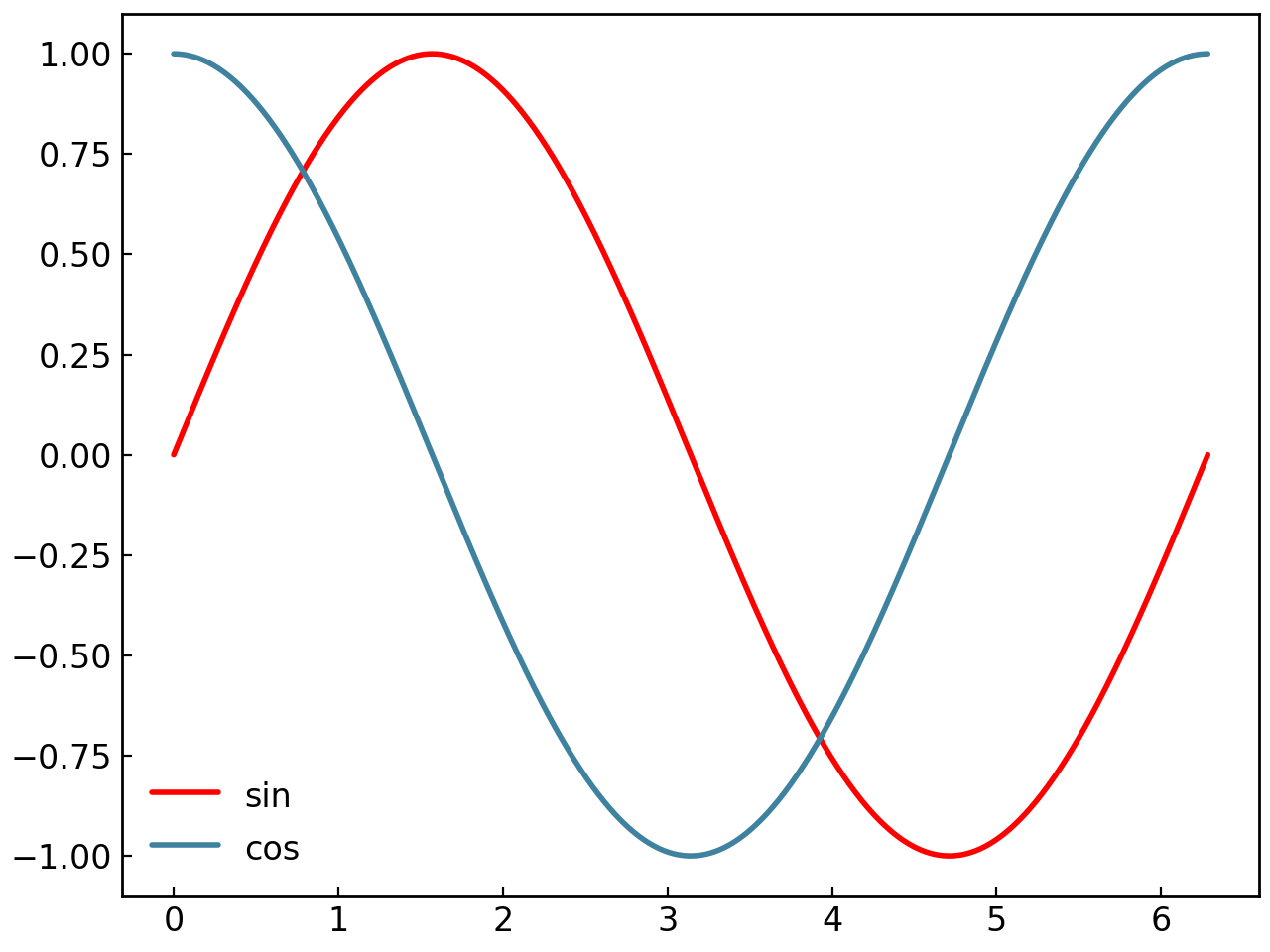
When creating a SmartFigure, you can pass elements directly:

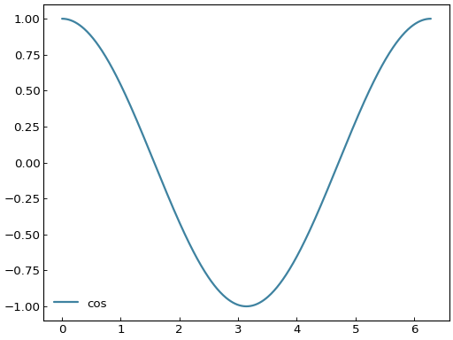
# For a 1x1 figure, all elements go to the single plot
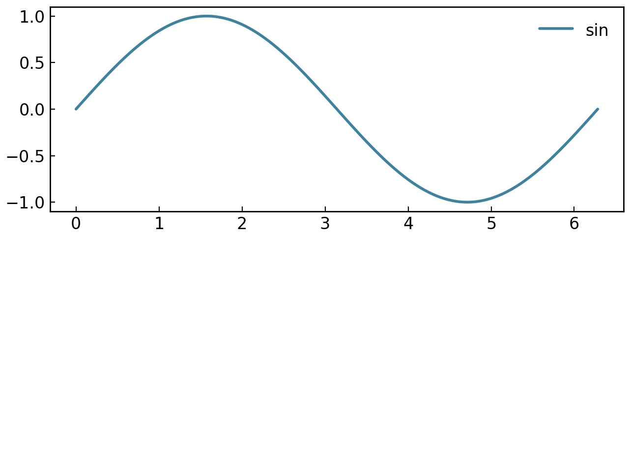
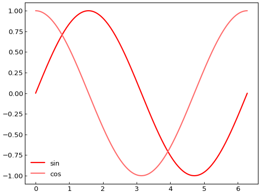
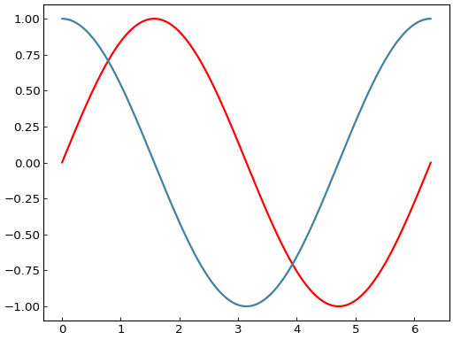
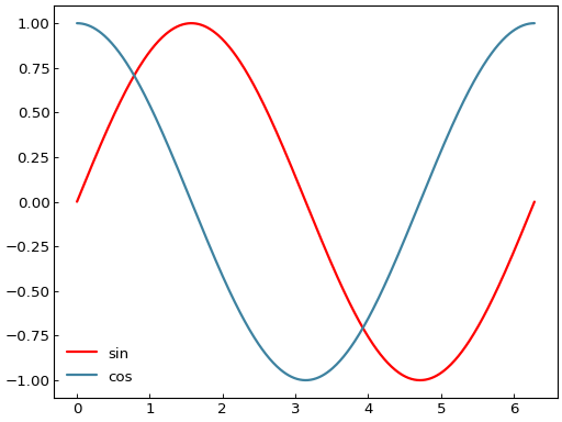
curve1 = gl.Curve.from_function(lambda x: np.sin(x), 0, 2*np.pi, label="sin")
curve2 = gl.Curve.from_function(lambda x: np.cos(x), 0, 2*np.pi, label="cos")

fig = gl.SmartFigure(elements=[curve1, curve2])
fig.show()

(png, hires.png, pdf)

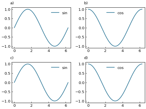
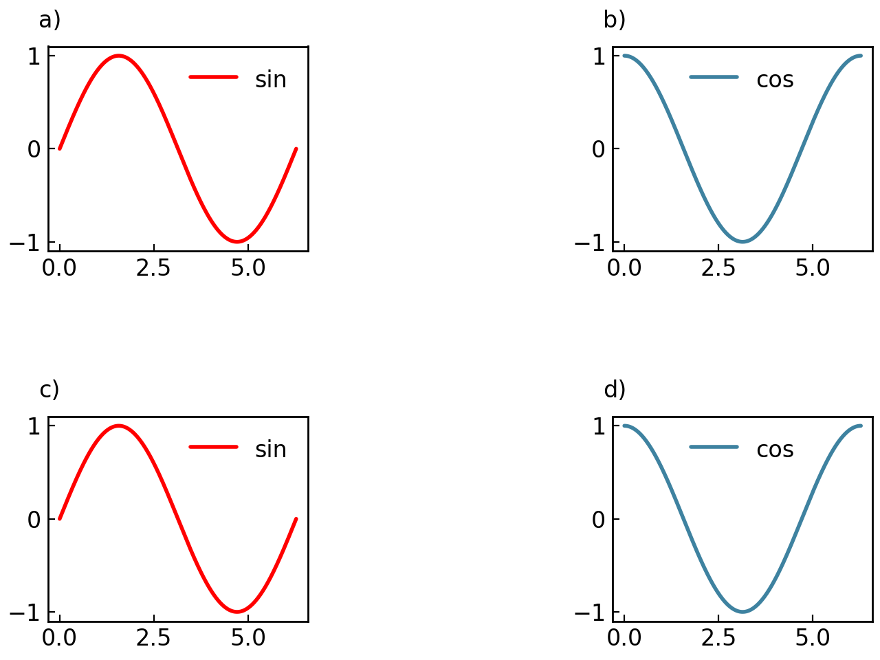
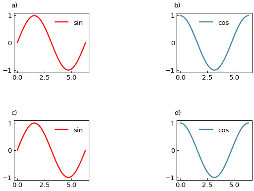
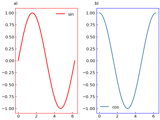
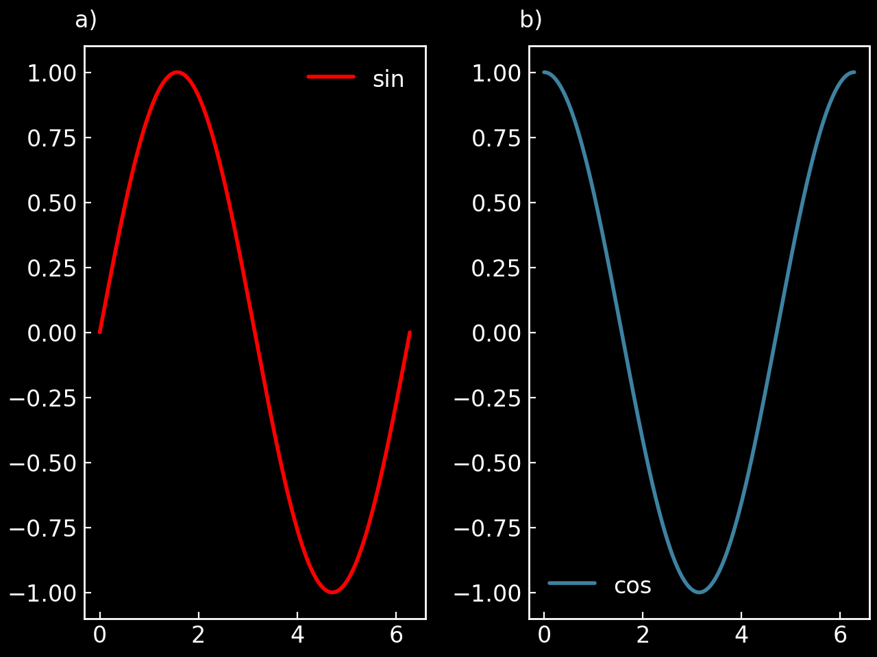
# For multi-subplot figures, each element fills one cell in order
fig = gl.SmartFigure(2, 2, elements=[curve1, curve2, curve1, curve2])
fig.show()

(png, hires.png, pdf)

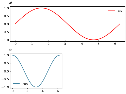
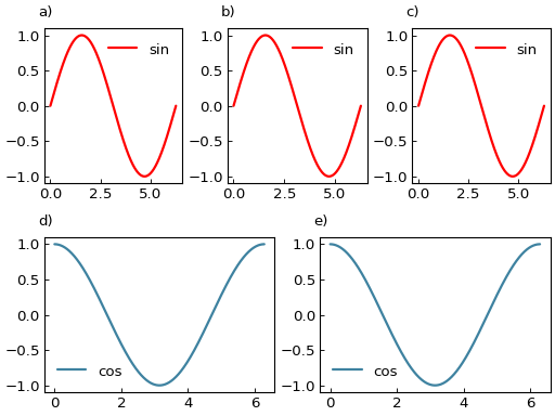
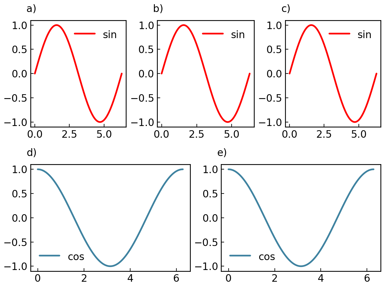
# You can also provide iterables of Plottables to create a child plot with multiple elements
fig = gl.SmartFigure(
    2, 2,
    elements=[
        [curve1, curve2],  # Both in the first child plot
        curve1,            # Second child plot
        None,              # Third position left empty
        [],                # Fourth child plot, drawn but empty
    ]
)
fig.show()

(png, hires.png, pdf)

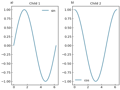
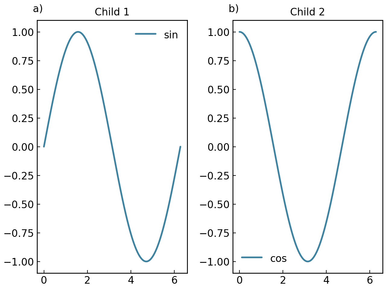
# You can also place existing SmartFigures directly in the layout
child1 = gl.SmartFigure(elements=curve1, title="Child 1")
child2 = gl.SmartFigure(elements=curve2, title="Child 2")

fig = gl.SmartFigure(1, 2, elements=[child1, child2])
fig.show()

(png, hires.png, pdf)

Method: add_elements()

The add_elements() method adds elements without replacing existing ones:

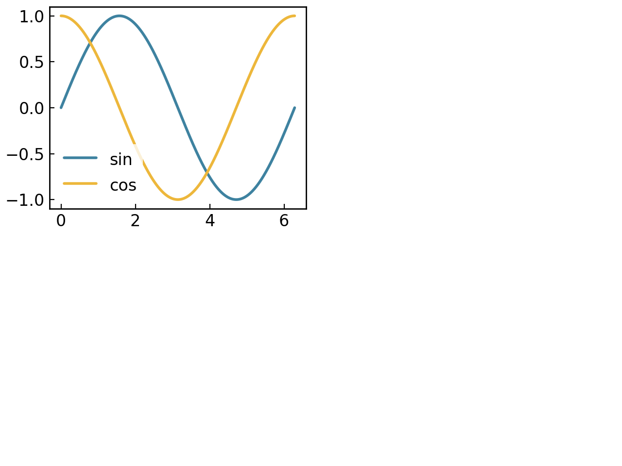
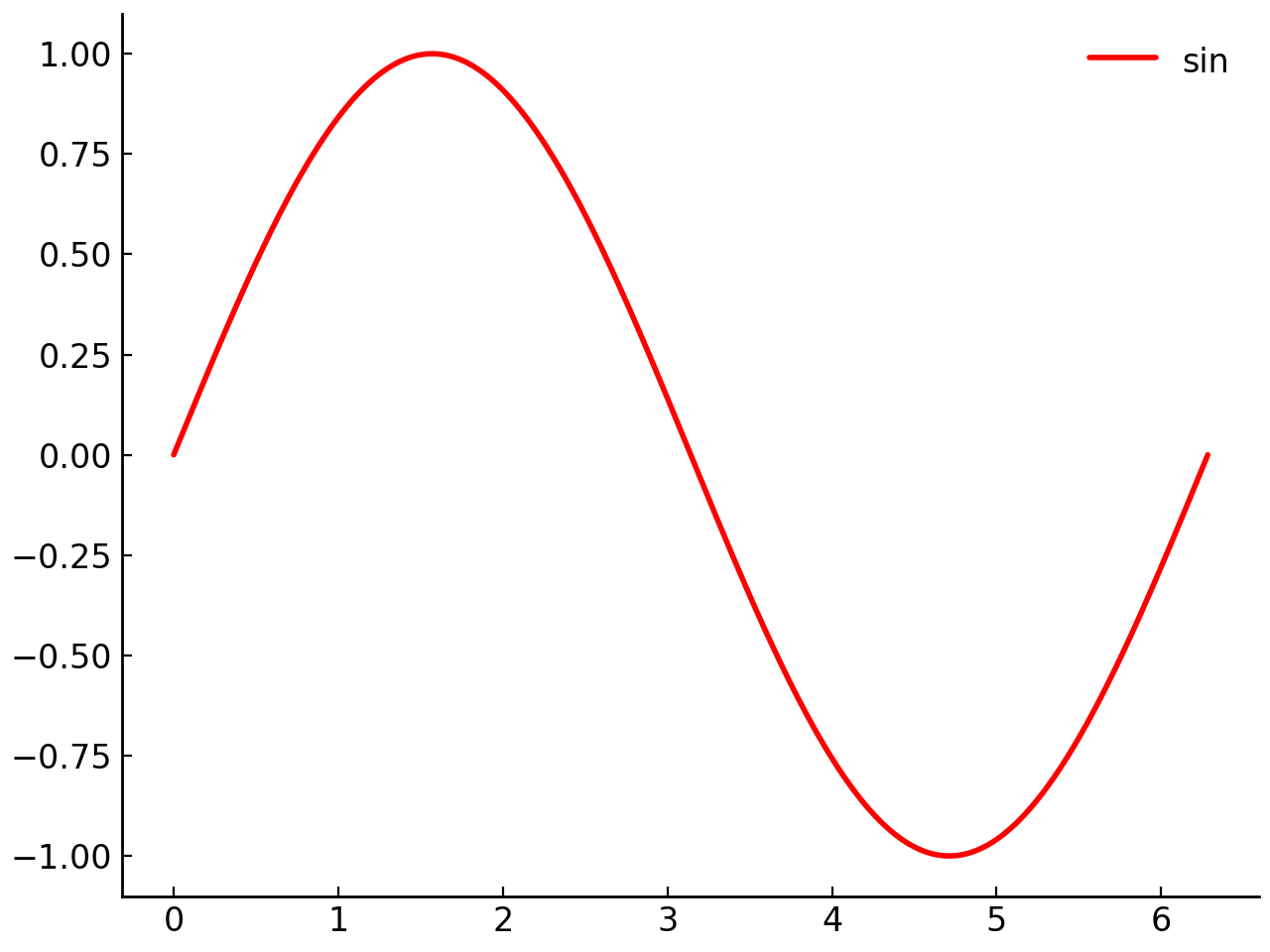
fig = gl.SmartFigure(elements=curve1)
fig.add_elements(curve2)  # Adds curve2 to the same subplot
fig.show()

(png, hires.png, pdf)

# For layouts, each argument is applied to the next grid position
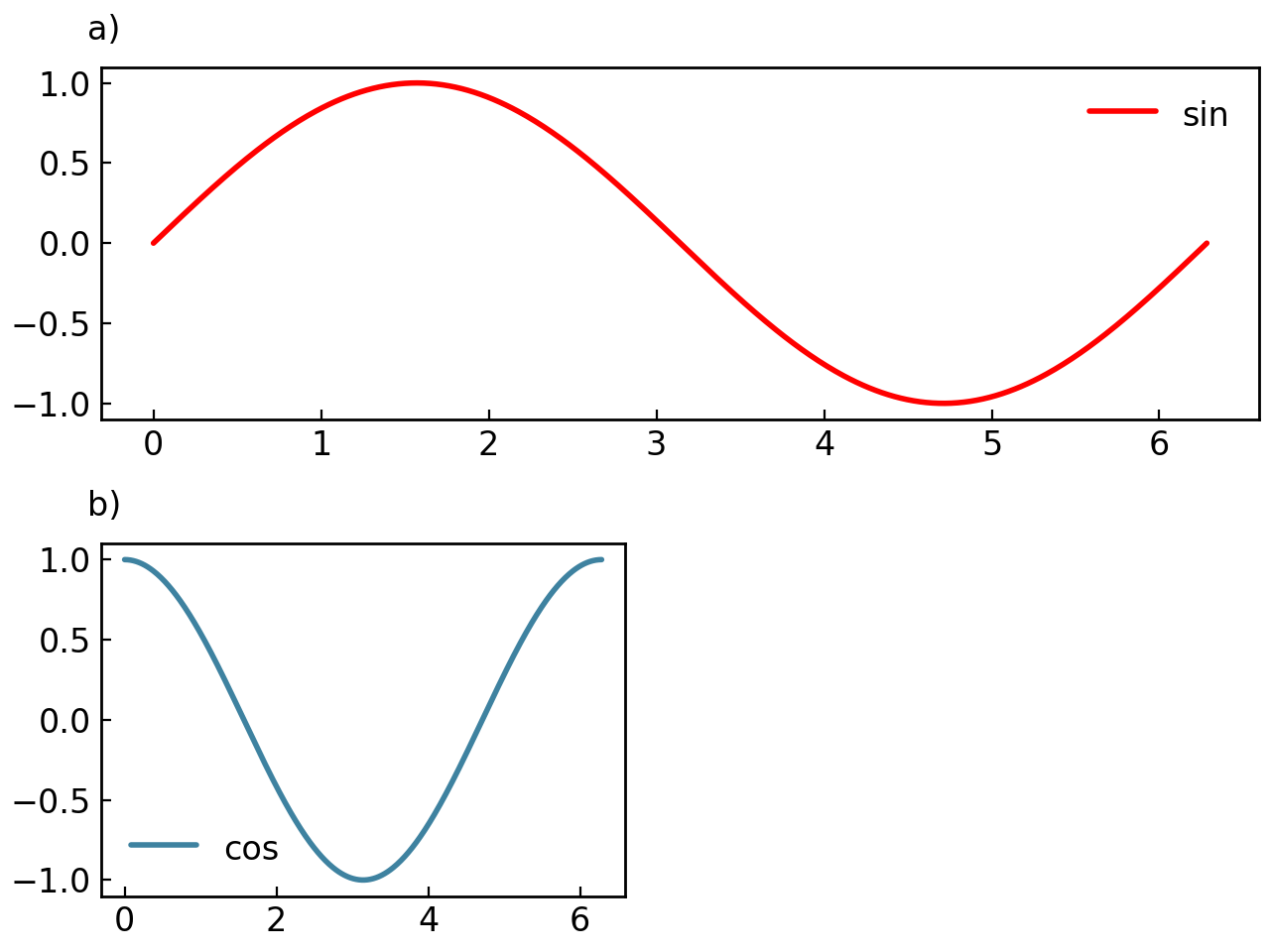
fig = gl.SmartFigure(2, 1)
fig.add_elements(curve1, curve2)  # Creates the two child plots
fig.show()

(png, hires.png, pdf)

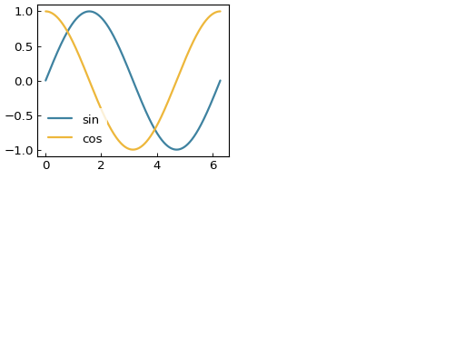
Similarly to the constructor, you can use iterables to specify multiple elements for the same plot:

fig = gl.SmartFigure(1, 2)
fig.add_elements([curve1, curve2], curve1.copy())
fig.show()

(png, hires.png, pdf)

When used on a layout, add_elements() walks through the grid from left to right, then top to bottom. If a child plot already exists in the targeted position, the new content is appended to it. If the position is empty, a new child plot is created there.

Property: elements

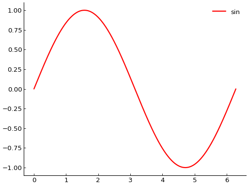
Setting the elements property replaces all existing elements:

fig = gl.SmartFigure(elements=curve1)
# This REPLACES curve1 with curve2
fig.elements = curve2
fig.show()

(png, hires.png, pdf)

Note

For multi-cell figures, the elements property fills the grid from left to right, then top to bottom. A Plottable or an iterable of Plottables creates a child plot in the corresponding cell. An existing SmartFigure can also be placed there directly.

Note

An existing child SmartFigure always occupies exactly one cell when it is placed through the elements property. Its num_rows and num_cols only describe its internal layout. If you want a child SmartFigure, a bare Plottable, or an iterable of Plottables to span multiple cells in the parent figure, use indexing with [] instead.

Note

Reading the elements property returns the SmartFigure’s current contents. For a single-plot SmartFigure, it returns the list of plotted Plottable objects. For a layout, it returns a list containing child SmartFigure objects or None placeholders for empty cells. A child spanning multiple cells appears only at its anchor position in that dense list.

Indexing using __setitem__

The most powerful method for element management uses indexing, which allows you to target specific positions in the layout and lets bare elements span multiple subplots:

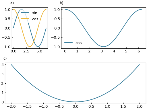
fig = gl.SmartFigure(2, 3)

# Add multiple elements to a child plot
fig[0, 0] = [curve1, curve2]

# Add element spanning multiple columns
fig[0, 1:] = curve2  # Spans columns 1 and 2 of row 0

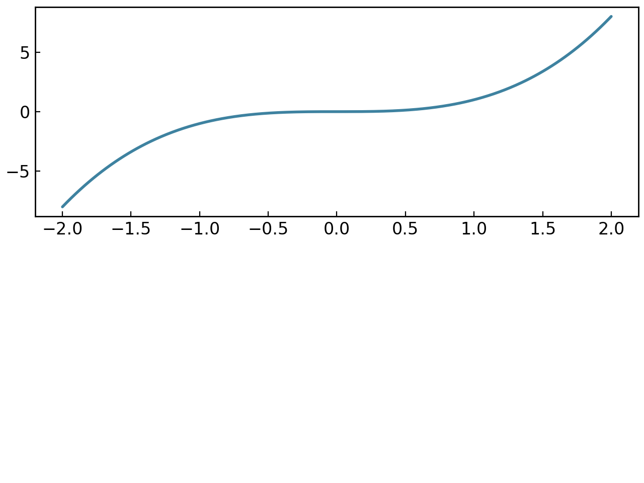
# Add element spanning entire row
fig[1, :] = gl.Curve.from_function(lambda x: x**2, -2, 2)

fig.show()

(png, hires.png, pdf)

# The += operator adds to the selected child plot
fig = gl.SmartFigure(2, 2)
fig[0, 0] = curve1
fig[0, 0] += curve2  # Adds curve2 without removing curve1
fig.show()

(png, hires.png, pdf)

Assigning a Plottable or an iterable of Plottables creates or updates a child plot. Assigning an existing SmartFigure inserts that figure as a nested child instead.

Understanding None and []

The distinction between these values is crucial for controlling how a position in the layout is drawn:

# None: Position is left empty
# [], [None] or any list with None: A child plot is created but drawn empty

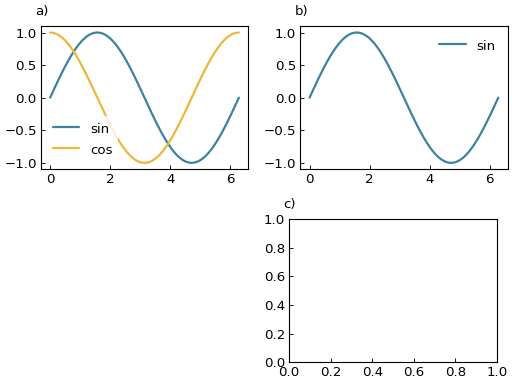
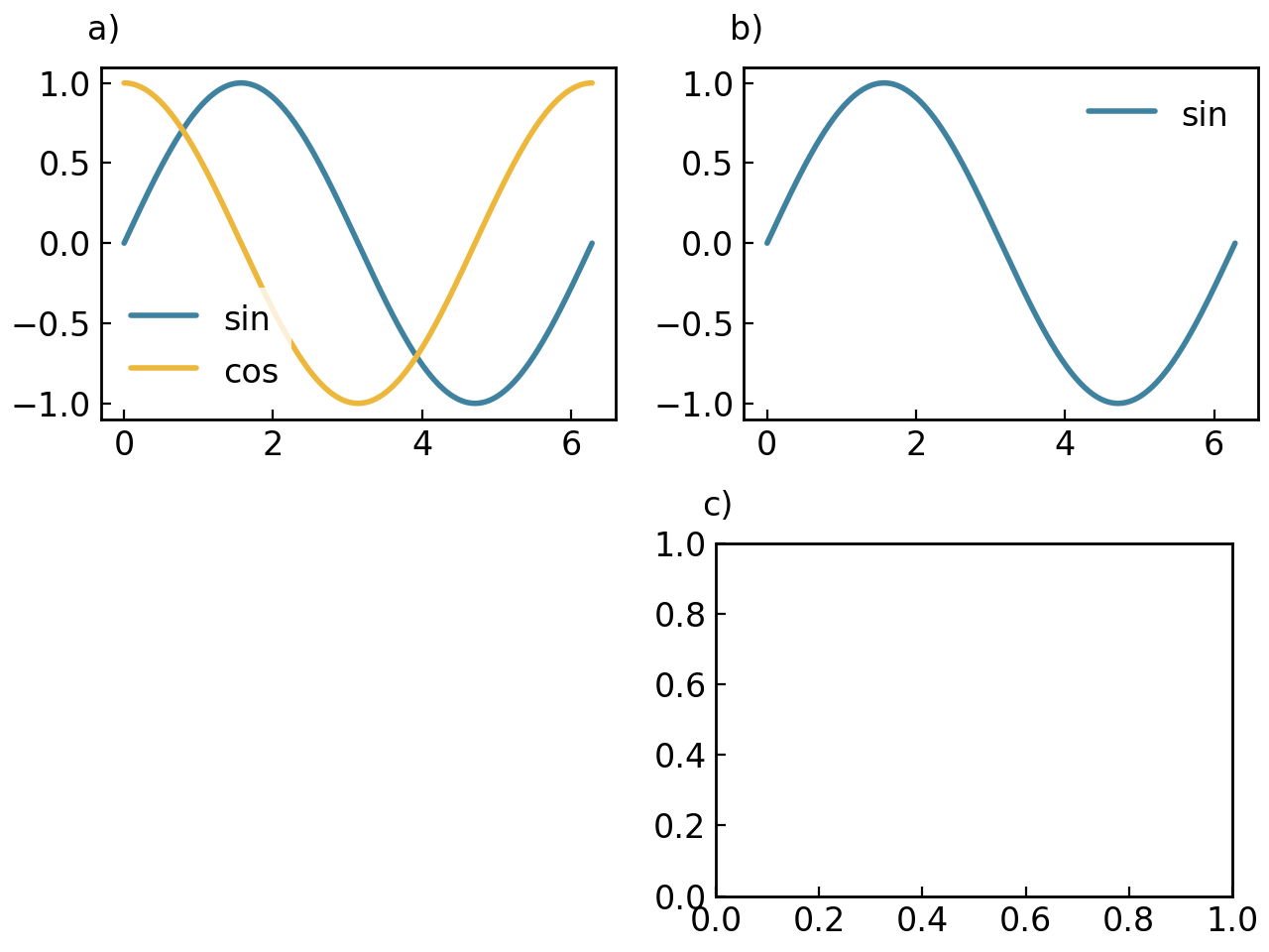
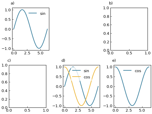
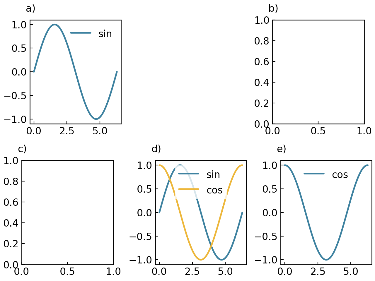
fig = gl.SmartFigure(2, 3, elements=[
    curve1,   # Normal child plot with element
    None,     # Empty position
    [None],   # Child plot created but empty
    [],       # Child plot created but empty (same as [None])
    [curve1, None, curve2],  # curve1 and curve2 plotted, None ignored
    curve2    # Normal child plot with element
])
fig.show()

(png, hires.png, pdf)

Removing Elements

To remove elements, set them to None:

fig = gl.SmartFigure(2, 2, elements=[curve1, curve2])
fig[1, :] = curve1  # Add spanning element

# Remove element from specific subplot
fig[0, 1] = None

# Remove multi-cell element - can use any cell it occupies
fig[1, 0] = None    # Removes the entire [1, :] element

fig.show()

(png, hires.png, pdf)

Note

When a multi-cell element is removed, you can delete it by clicking on any cell it occupies. For example, if an element spans [1, :] (the entire second row), you can remove it with fig[1, 0] = None, fig[1, 1] = None, or fig[1, :] = None.

Retrieving Elements

You can retrieve child plots using indexing. Indexing returns the SmartFigure occupying the requested position:

fig = gl.SmartFigure(2, 2)
fig[0, 0] = [curve1, curve2]
fig[1, 0] = curve1
child = fig[0, 0]
curves = child.elements  # Returns [curve1, curve2]
single_curve = fig[1, 0].elements[0]  # Returns curve1

You can then modify that child plot directly:

fig = gl.SmartFigure(1, 2, elements=[[curve1.copy()], [curve2.copy()]])

child = fig[0, 0]
child += curve2.copy()
fig[0, 1].add_elements(curve1.copy())

fig.show()

(png, hires.png, pdf)

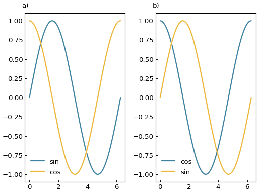
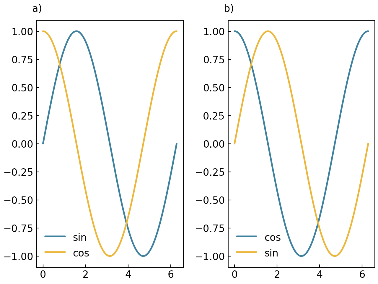
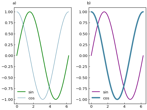
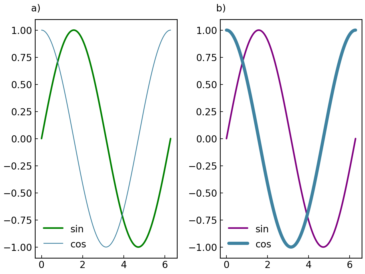
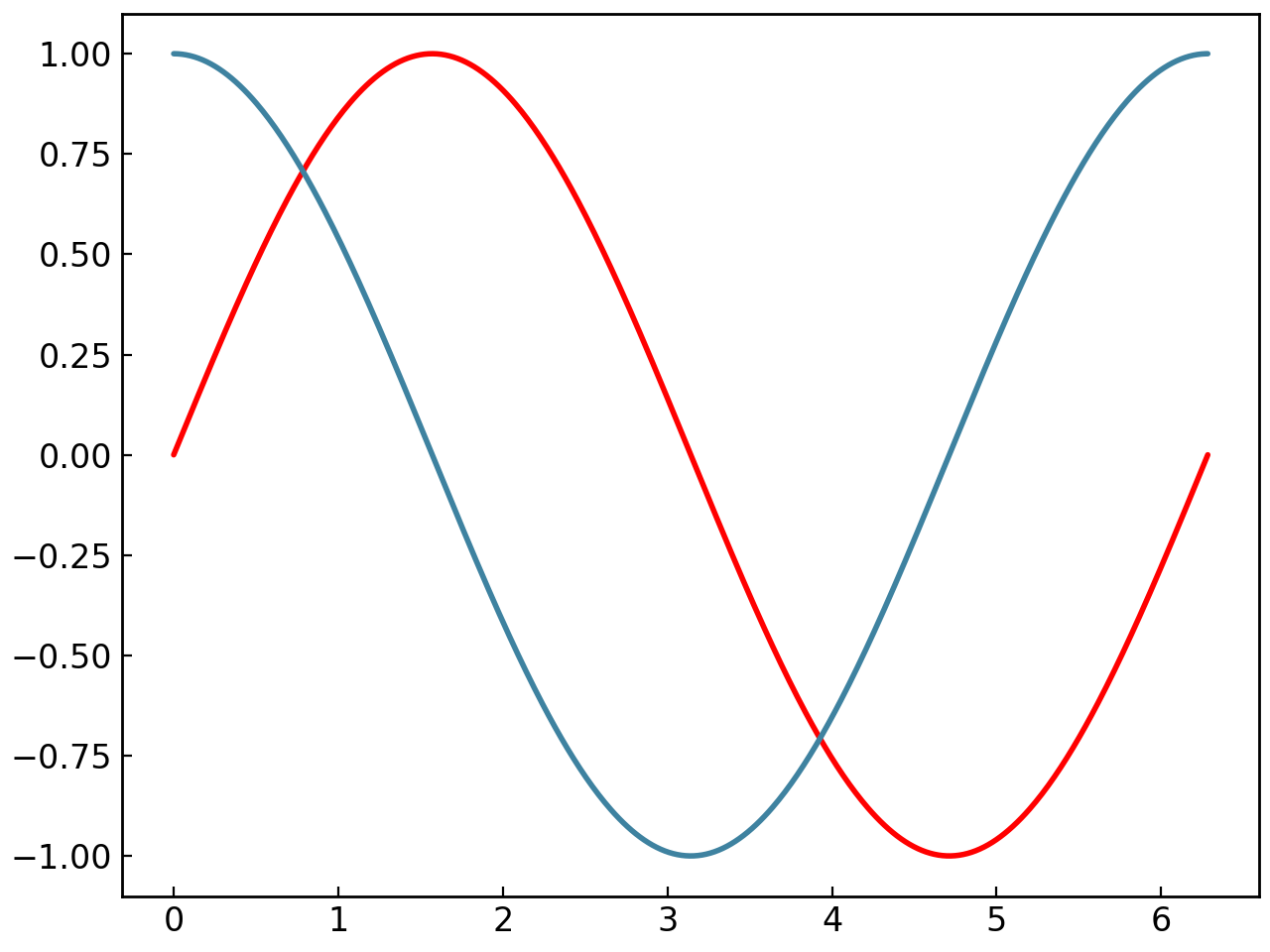
You can also iterate on the SmartFigure directly to access each child plot in order:

fig = gl.SmartFigure(1, 2, elements=[[curve1.copy(), curve2.copy()], [curve1.copy(), curve2.copy()]])

colors = ["green", "purple"]
line_widths = [1, 4]
for child_plot, color, line_width in zip(fig, colors, line_widths):
    child_plot.elements[0].color = color
    child_plot.elements[1].line_width = line_width

fig.show()

(png, hires.png, pdf)

Accessing Multi-Cell Elements

One of the most powerful features of SmartFigure is the ability to access and modify elements that span multiple cells by clicking on any cell they occupy:

# Create a figure with a multi-cell element spanning the entire first row
fig = gl.SmartFigure(2, 3)
fig[0, :] = curve1  # Spans all three columns of row 0
fig.show()

# You can access this child plot via any cell it occupies
child_via_col0 = fig[0, 0]
child_via_col1 = fig[0, 1]
child_via_col2 = fig[0, 2]
child_via_slice1 = fig[0, 1:]
child_via_slice2 = fig[0, :]

(png, hires.png, pdf)

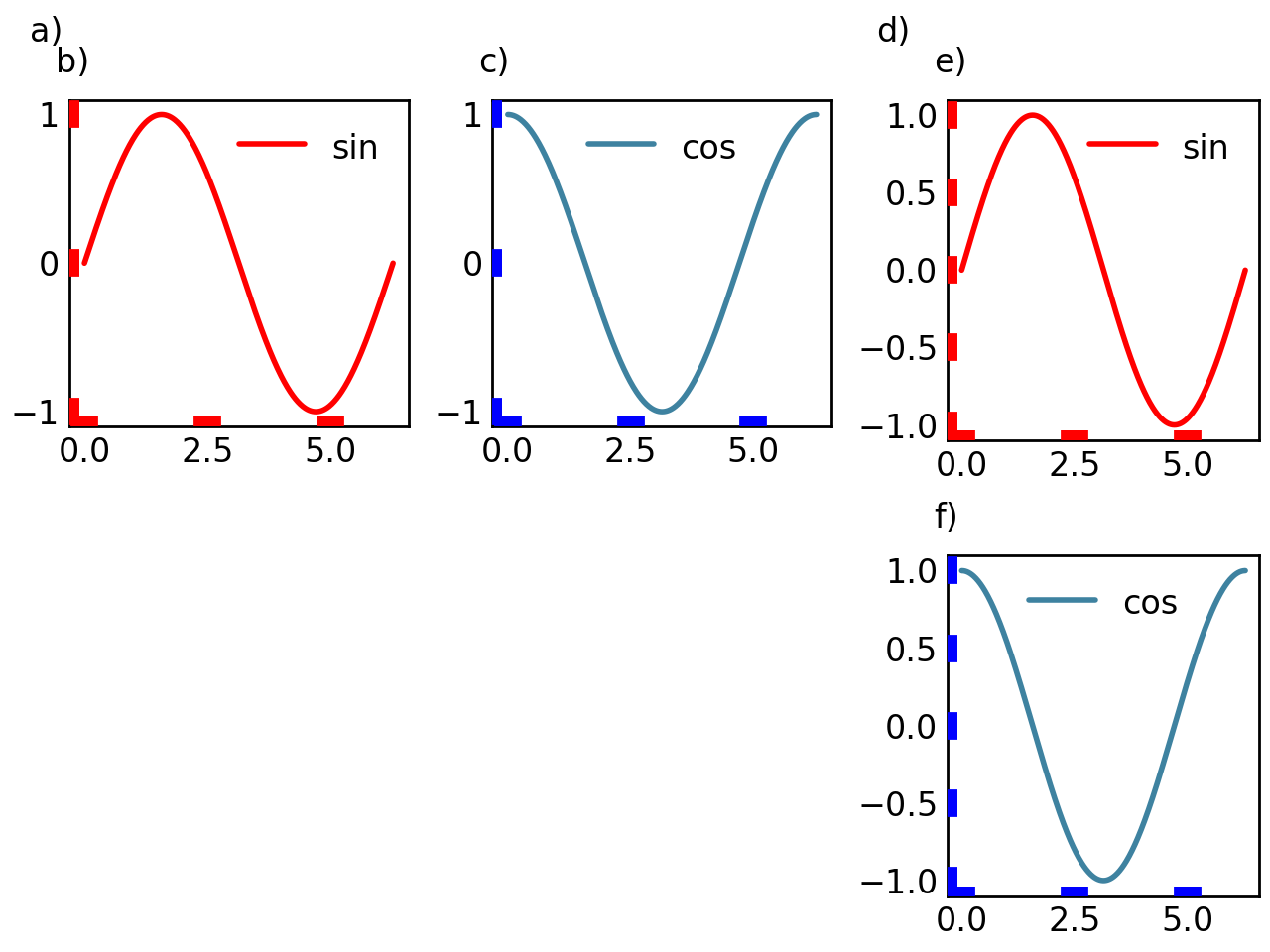
This makes it much more intuitive to work with complex layouts:

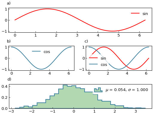
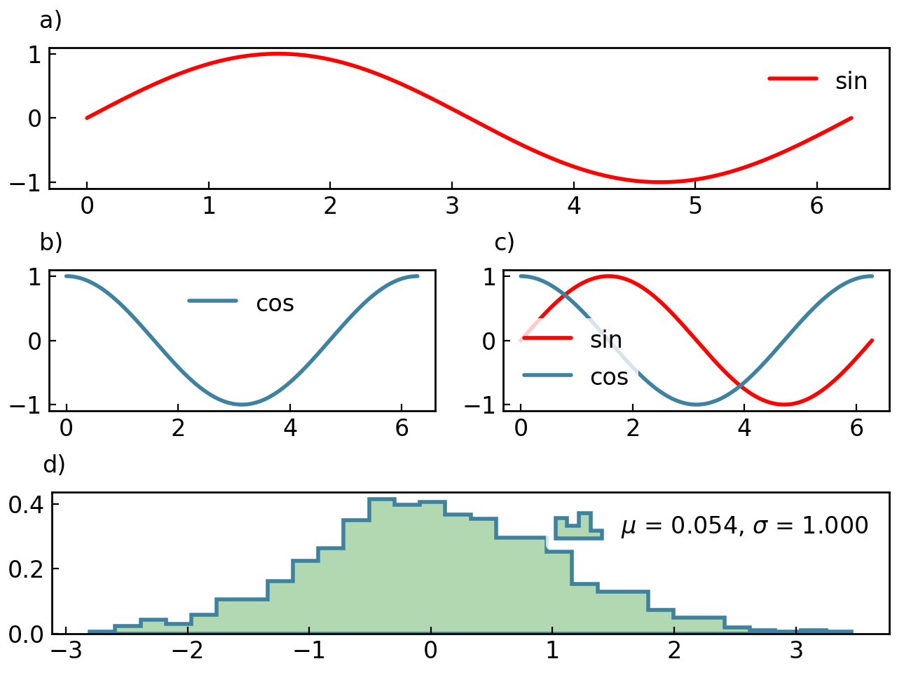
fig = gl.SmartFigure(3, 2)

# Add elements with different spans
fig[0, :] = curve1     # Top row, spans both columns
fig[1, 0] = curve2     # Middle left, single cell
fig[1, 1] = [curve1, curve2]  # Middle right, single cell with multiple elements
fig[2, :] = gl.Histogram(np.random.randn(1000), bins=30)  # Bottom row, spans both columns

# Access and modify via clicking on any cell
fig[0, 0].elements[0].color = "red"  # Modify top row element via first column
fig[2, 1].elements[0].face_color = "green"  # Modify bottom histogram via second column

fig.show()

(png, hires.png, pdf)

Warning

The only rule that needs to be followed is that you cannot access or modify elements using a slice that overlaps with multiple different subplots. Therefore, you must always use a slice that includes at most a single drawn subfigure.

fig = gl.SmartFigure(2, 2)
fig[0, :] = curve1  # Spans entire first row
fig[1, 0] = curve2  # Single cell in second row
fig.show()

# This raises an error - slice overlaps with two different child plots
try:
    element = fig[0:2, :]
except gl.GraphingException:
    print("Cannot access multiple different elements with one slice")

(png, hires.png, pdf)

When you replace a multi-cell element, the new element will inherit the span of the original element:

fig = gl.SmartFigure(2, 3)
fig[0, :] = curve1  # Spans entire first row

# Replace via single cell - new element inherits [0, :] span
fig[0, 1] = curve2

# curve2 now spans the entire first row
assert fig[0, 0] is fig[0, 1]  # Same child plot

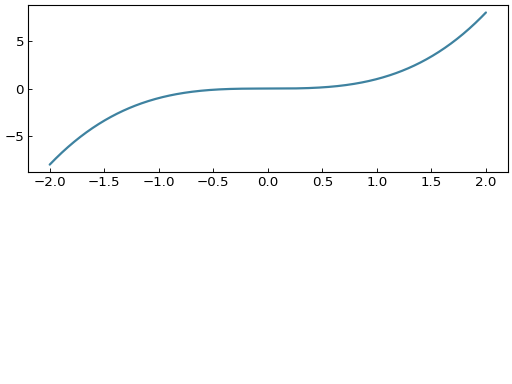
# Replace via slice - new element inherits [0, :] span
fig[0, 0:2] = gl.Curve.from_function(lambda x: x**3, -2, 2)

fig.show()

(png, hires.png, pdf)

This behavior makes it intuitive to replace or add elements while maintaining your layout structure.

Layout and Structure Control

Grid System

The SmartFigure uses a grid system defined by num_rows and num_cols:

# 2x3 grid creates 6 possible subplot positions
fig = gl.SmartFigure(num_rows=2, num_cols=3)

# Can also use the shape property
fig.shape = (3, 2)  # Now 3x2 grid
fig.elements = [[]]*6
fig.show()

(png, hires.png, pdf)

Note

Changing the num_rows or num_cols of a preexisting SmartFigure is only allowed if there are no elements in the rows/columns being removed. If the SmartFigure was previously being used as a single plot, increasing num_rows or num_cols turns it into a layout and moves the original plot to the top-left position.

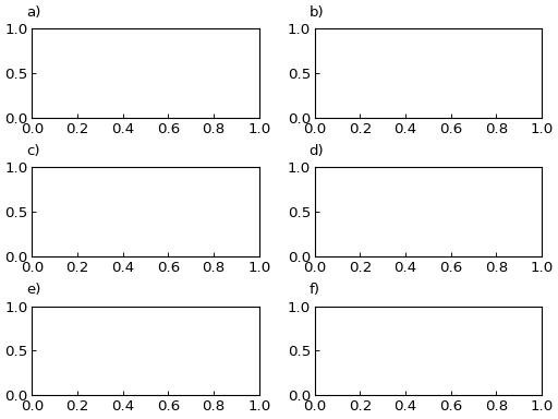
This grid system can be exploited to create complex layouts by adding elements that span multiple rows or columns:

# 4 column layout that appears like a 2 column layout
fig = gl.SmartFigure(num_rows=2, num_cols=4)
fig[0, :2] = curve1
fig[0, 2:] = curve1
fig[1, 1:3] = curve2  # places in the middle of the bottom row
fig.show()

(png, hires.png, pdf)

# 6 column layout that appears like a 3 and 2 column layout
fig = gl.SmartFigure(num_rows=2, num_cols=6)
fig[0, :2] = curve1
fig[0, 2:4] = curve1
fig[0, 4:] = curve1
fig[1, :3] = curve2
fig[1, 3:] = curve2
fig.show()

(png, hires.png, pdf)

Figure Size

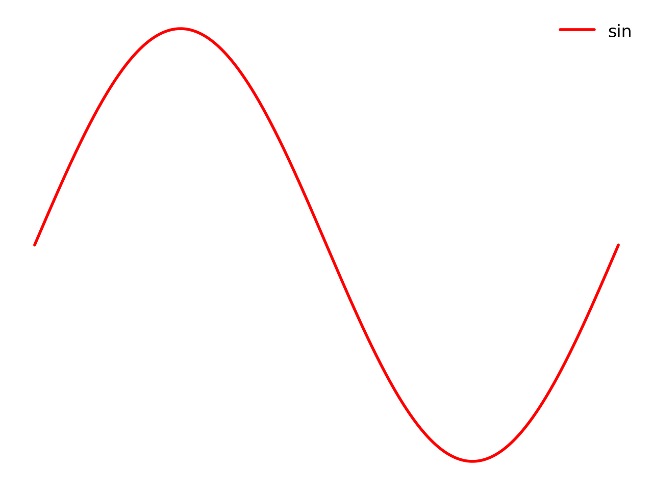
Control the overall figure size with the size parameter:

# Size in inches (width, height)
fig = gl.SmartFigure(size=(10, 6), elements=curve1)
fig.show()

(png, hires.png, pdf)

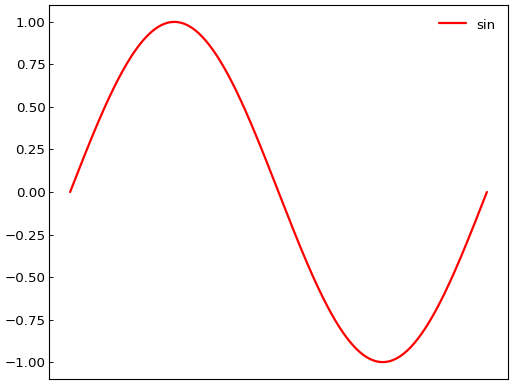
# Use INHERIT to let the style file determine the size
fig = gl.SmartFigure(size=gl.INHERIT, elements=curve1)
fig.show()

(png, hires.png, pdf)

Note

When a SmartFigure is nested inside another, its size parameter is ignored and determined by the parent figure’s size and layout.

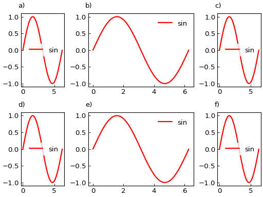
Padding Between Subplots

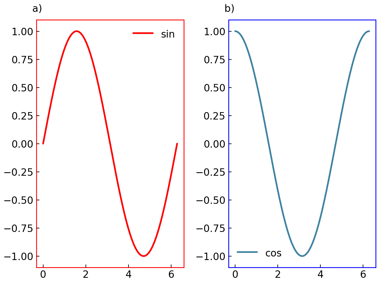
Control spacing between subplots with width_padding and height_padding:

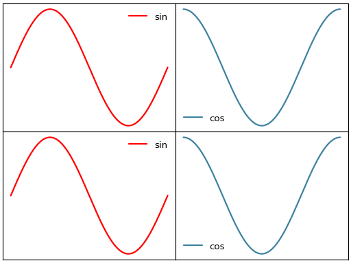
# More padding
fig = gl.SmartFigure(
    2, 2,
    width_padding=0.2,
    height_padding=0.1,
    elements=[curve1, curve2, curve1, curve2]
)
fig.show()

(png, hires.png, pdf)

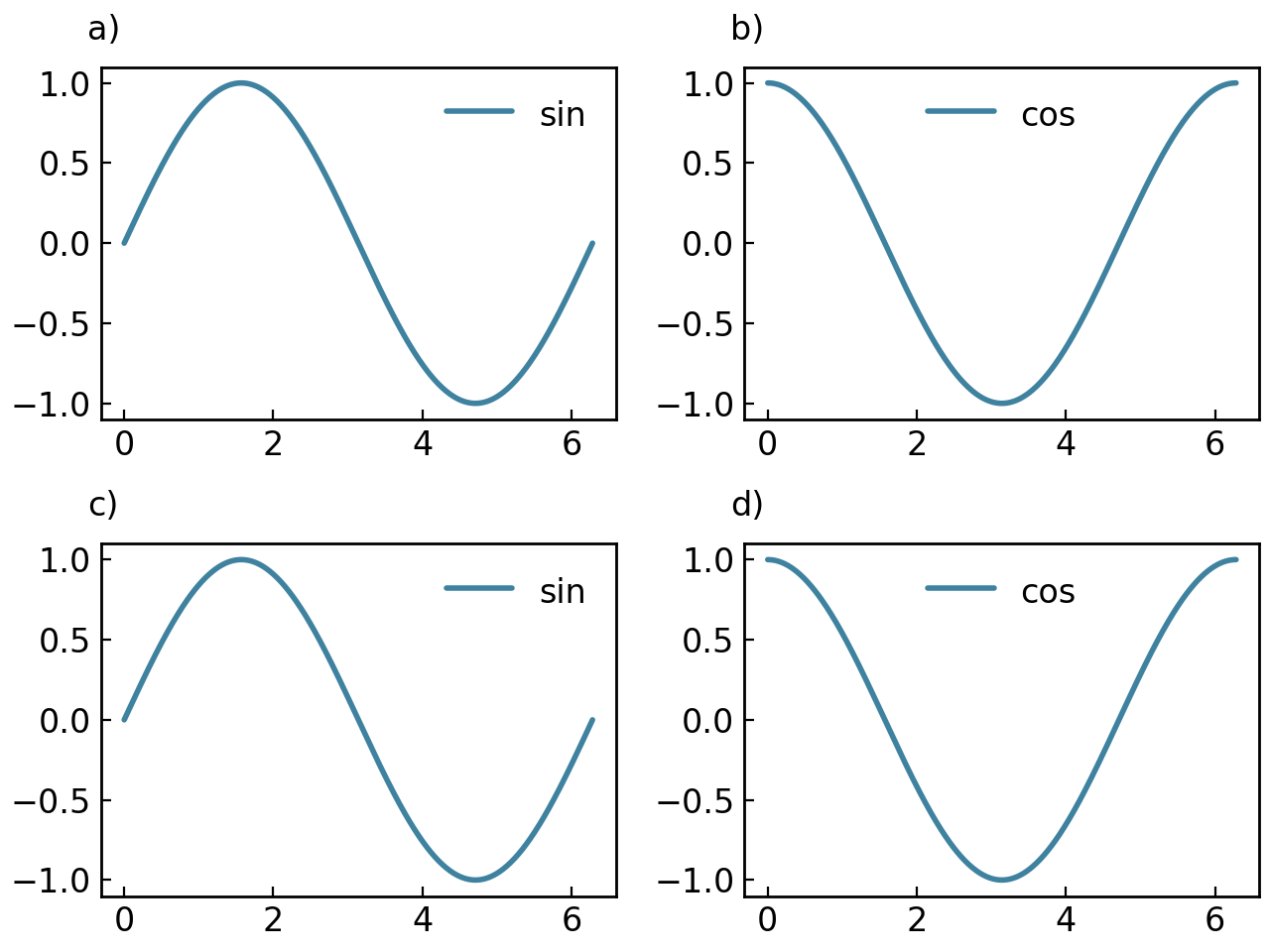
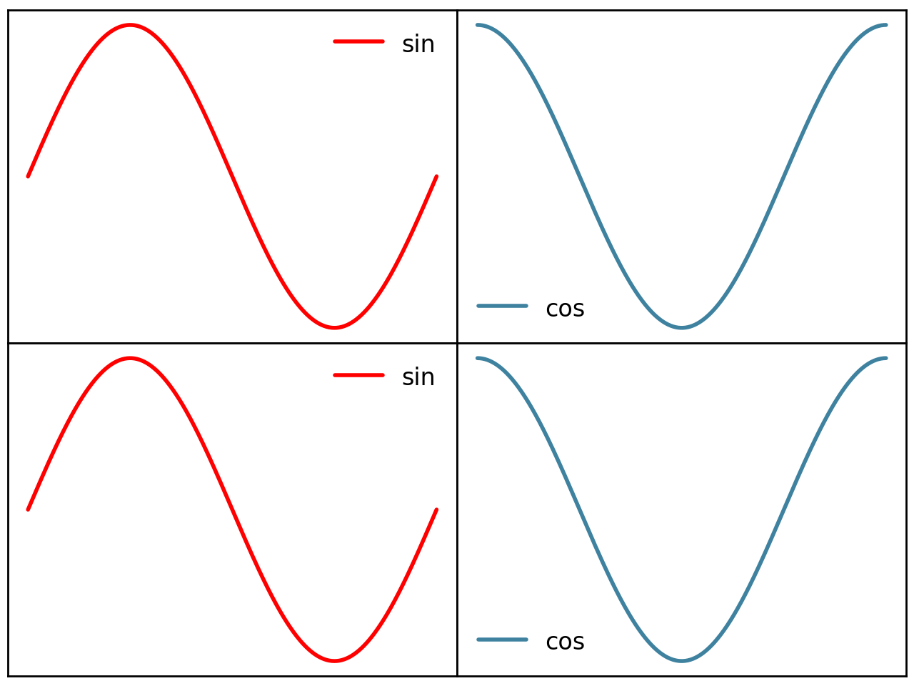
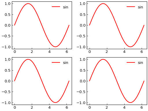
# No padding (compact layout)
fig = gl.SmartFigure(
    2, 2,
    width_padding=0,
    height_padding=0,
    remove_x_ticks=True,
    remove_y_ticks=True,
    reference_labels=False,
    elements=[curve1, curve2, curve1, curve2]
)
fig.show()

(png, hires.png, pdf)

Subplot Size Ratios

Control relative sizes of rows and columns with width_ratios and height_ratios:

# Make middle column twice as wide as others
fig = gl.SmartFigure(
    2, 3,
    width_ratios=[1, 2, 1],
    height_ratios=[1, 1],
    elements=[curve1]*6
)
fig.show()

(png, hires.png, pdf)

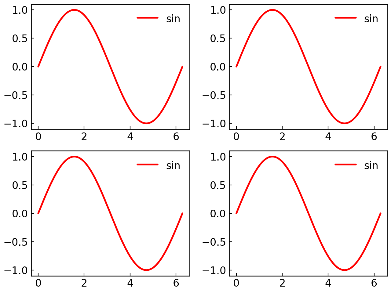
# Make first row taller
fig = gl.SmartFigure(
    2, 2,
    height_ratios=[2, 1],
    elements=[curve1]*4
)
fig.show()

(png, hires.png, pdf)

Axes Configuration

Labels and Titles

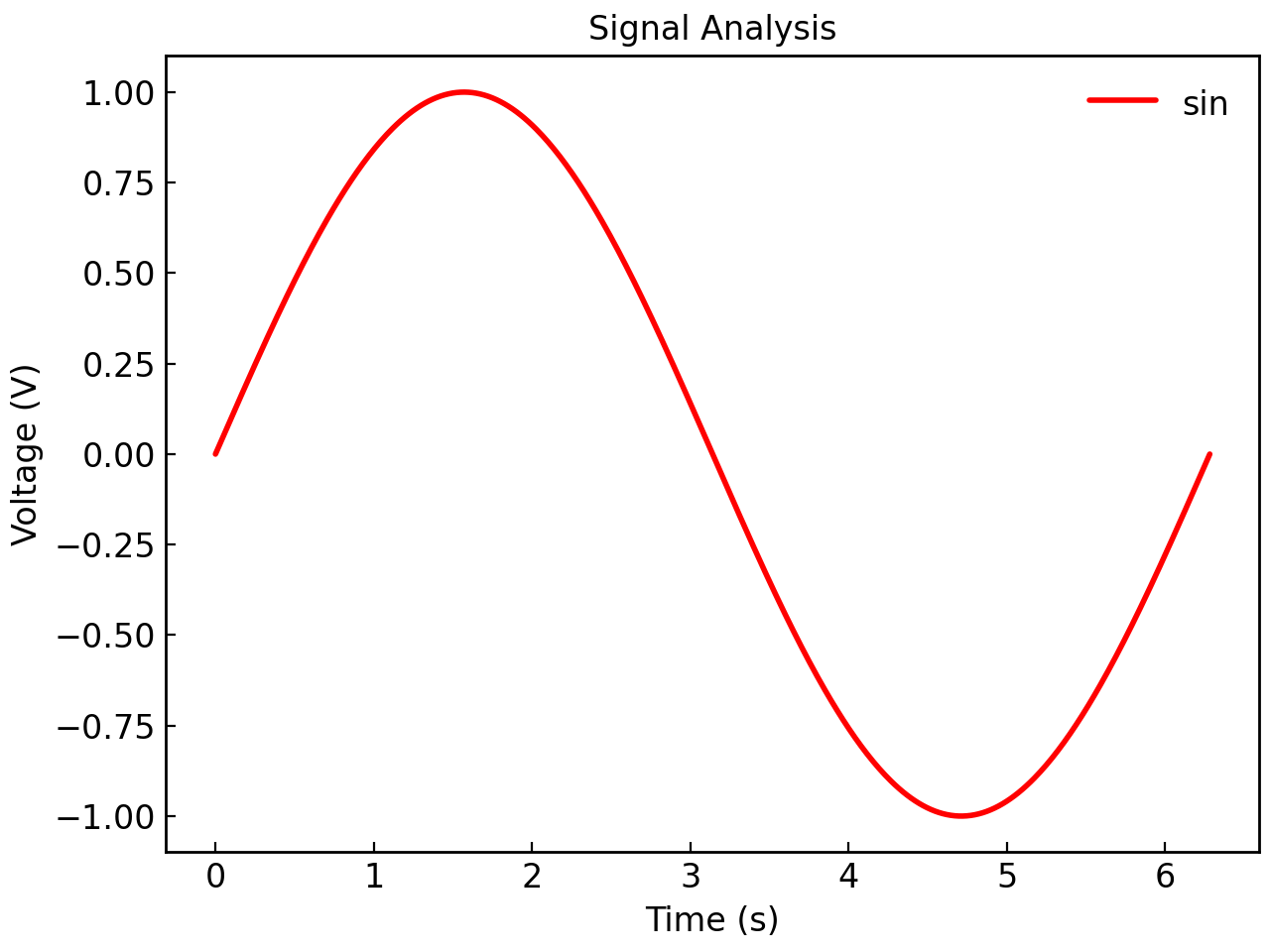
Main Figure Labels

Set labels for the entire figure:

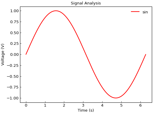
fig = gl.SmartFigure(
    x_label="Time (s)",
    y_label="Voltage (V)",
    title="Signal Analysis",
    elements=curve1,
)
fig.show()

(png, hires.png, pdf)

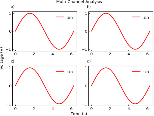
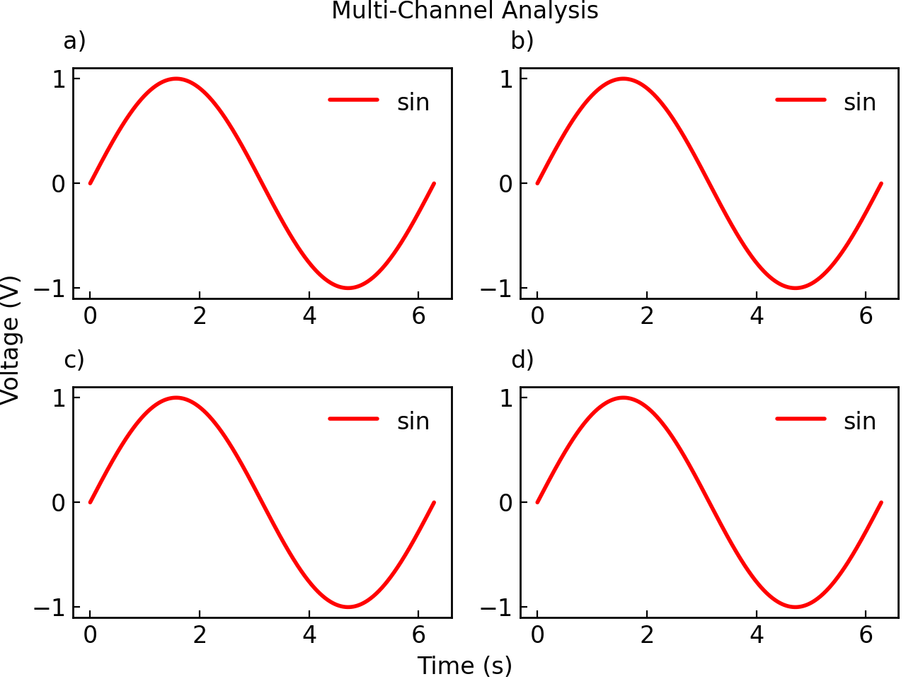
# For multi-subplot figures, labels apply to all subplots
fig = gl.SmartFigure(
    2, 2,
    x_label="Time (s)",
    y_label="Voltage (V)",
    title="Multi-Channel Analysis",
    elements=[curve1]*4
)
fig.show()

(png, hires.png, pdf)

Individual Subplot Labels

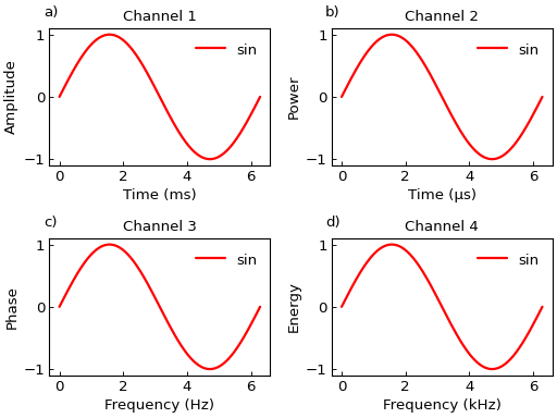
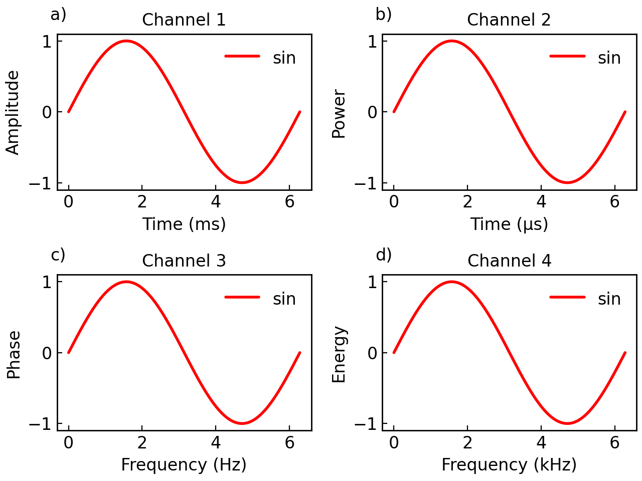
Use sub_x_labels, sub_y_labels, and subtitles for per-subplot customization:

fig = gl.SmartFigure(
    2, 2,
    sub_x_labels=["Time (ms)", "Time (μs)", "Frequency (Hz)", "Frequency (kHz)"],
    sub_y_labels=["Amplitude", "Power", "Phase", "Energy"],
    subtitles=["Channel 1", "Channel 2", "Channel 3", "Channel 4"],
    elements=[curve1]*4
)
fig.show()

(png, hires.png, pdf)

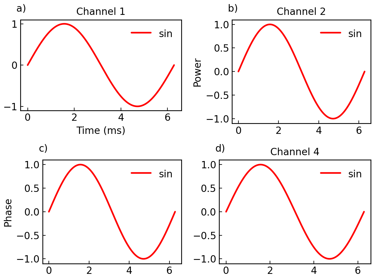
You can also use None in the lists to skip labels for specific subplots, or give shorter lists:

fig = gl.SmartFigure(
    2, 2,
    sub_x_labels=["Time (ms)"],  # Only first subplot gets x label
    sub_y_labels=[None, "Power", "Phase"],  # Last subplot uses default y label
    subtitles=["Channel 1", "Channel 2", None, "Channel 4"],  # Skip third subtitle
    elements=[curve1]*4
)
fig.show()

(png, hires.png, pdf)

Warning

If the provided lists are longer than the number of subfigures drawn by the SmartFigure, an error will be raised. For details on list length rules, see the List Length and Padding Rules section.

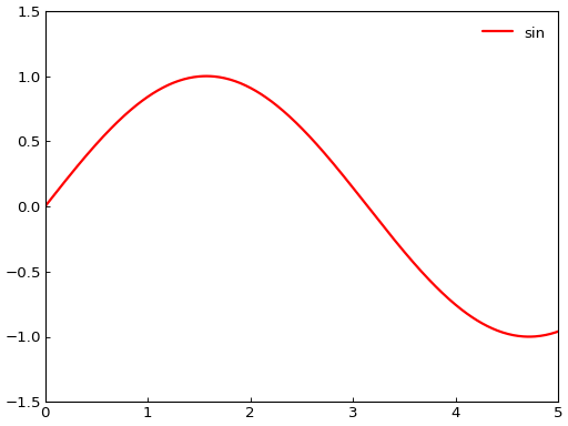
Axes Limits

Set axis limits for all subplots:

fig = gl.SmartFigure(
    x_lim=(0, 5),
    y_lim=(-1.5, 1.5),
    elements=curve1,
)
fig.show()

(png, hires.png, pdf)

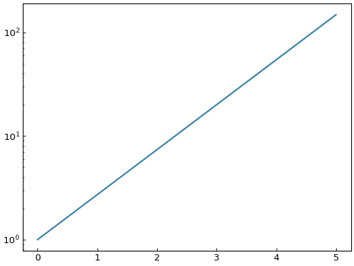
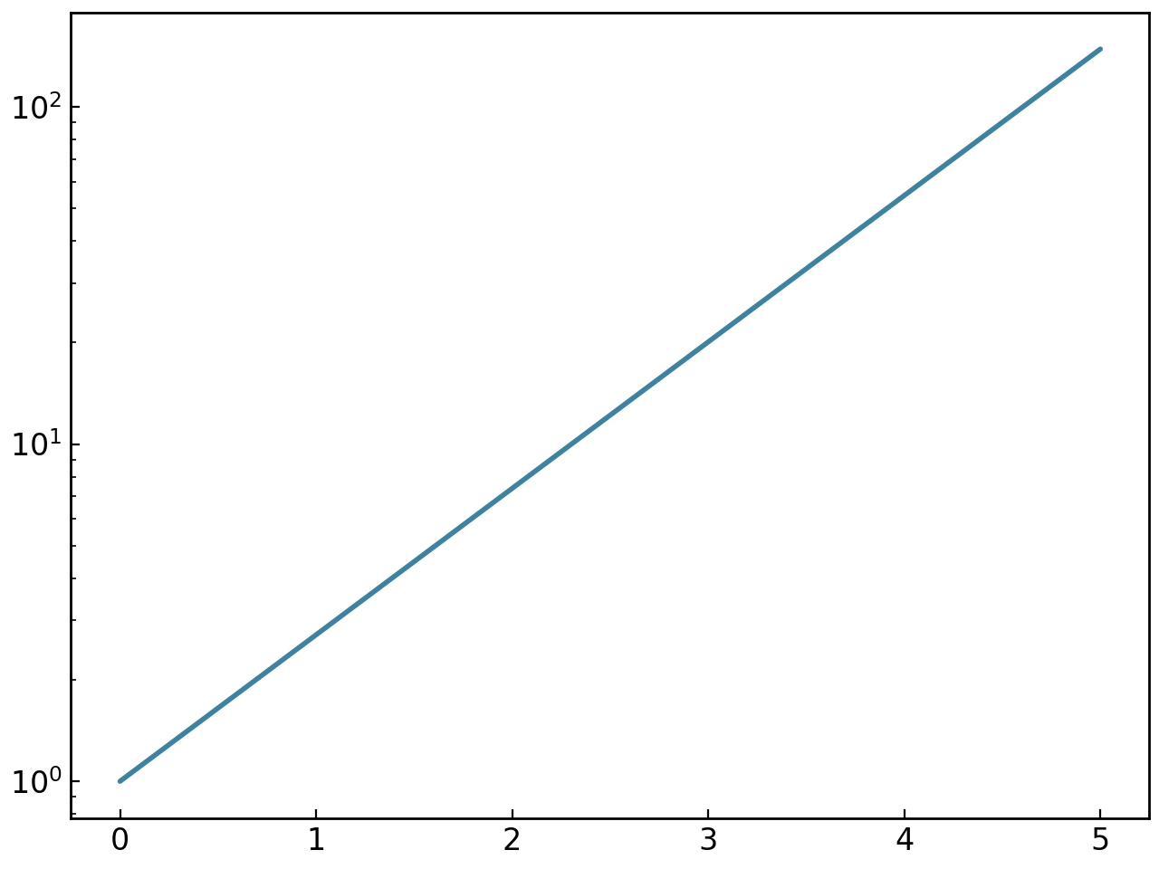
Logarithmic Scales

Enable logarithmic scales:

exp_curve = gl.Curve.from_function(lambda x: np.exp(x), 0, 5)

fig = gl.SmartFigure(
    log_scale_x=False,
    log_scale_y=True,
    elements=exp_curve,
)
fig.show()

(png, hires.png, pdf)

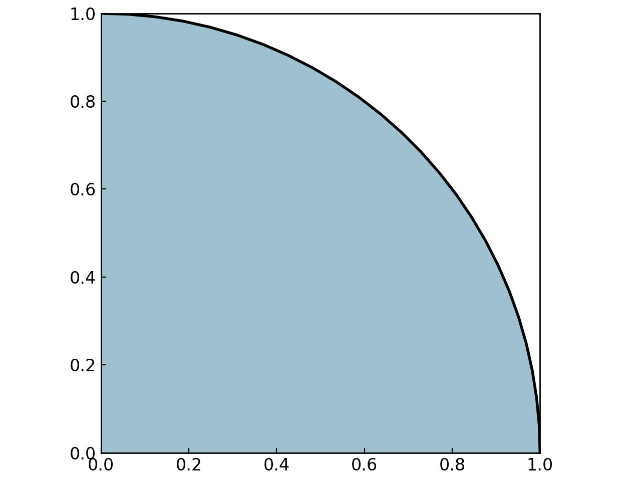
Aspect Ratios

Control aspect ratio of the data and the plot box:

# aspect_ratio controls data aspect ratio
circle = gl.Circle(0, 0, 1)

fig = gl.SmartFigure(
    aspect_ratio="equal",  # Makes circle truly circular
    elements=circle,
)
fig.show()

(png, hires.png, pdf)

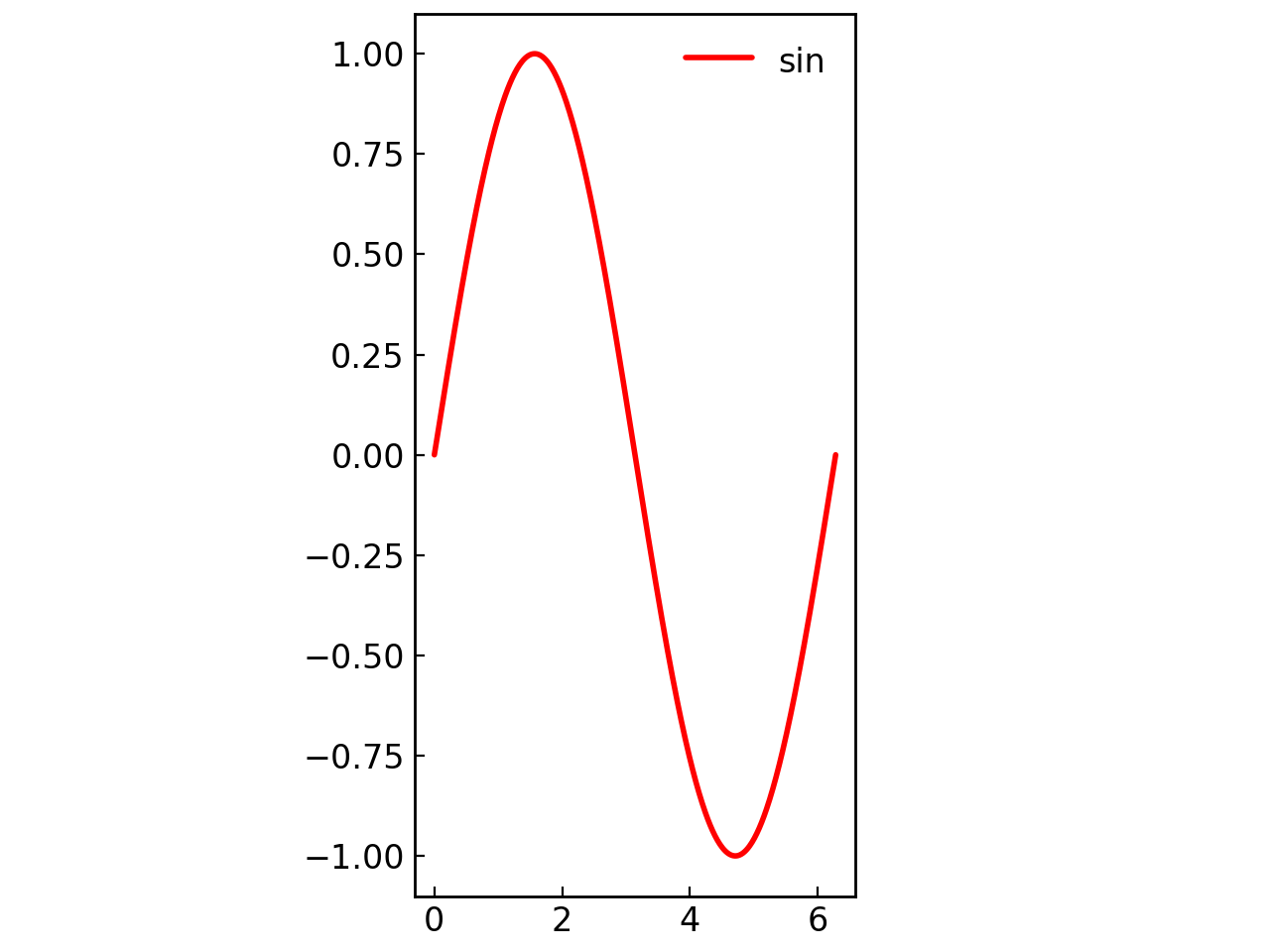
# box_aspect_ratio controls the plot box shape
fig = gl.SmartFigure(
    box_aspect_ratio=2.0,  # Box is twice as tall as wide
    elements=curve1,
)
fig.show()

(png, hires.png, pdf)

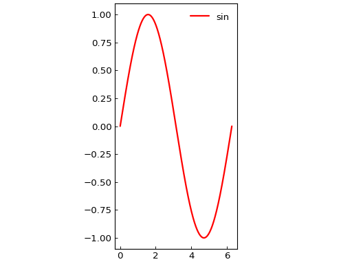
Warning

Do not confuse aspect_ratio (data aspect) with box_aspect_ratio (box shape). aspect_ratio affects how data is displayed within the axes (e.g. the aspect ratio of the pixels if plotting a Heatmap), while box_aspect_ratio changes the physical size of the axes box.

Inverting Axes

Invert axes direction:

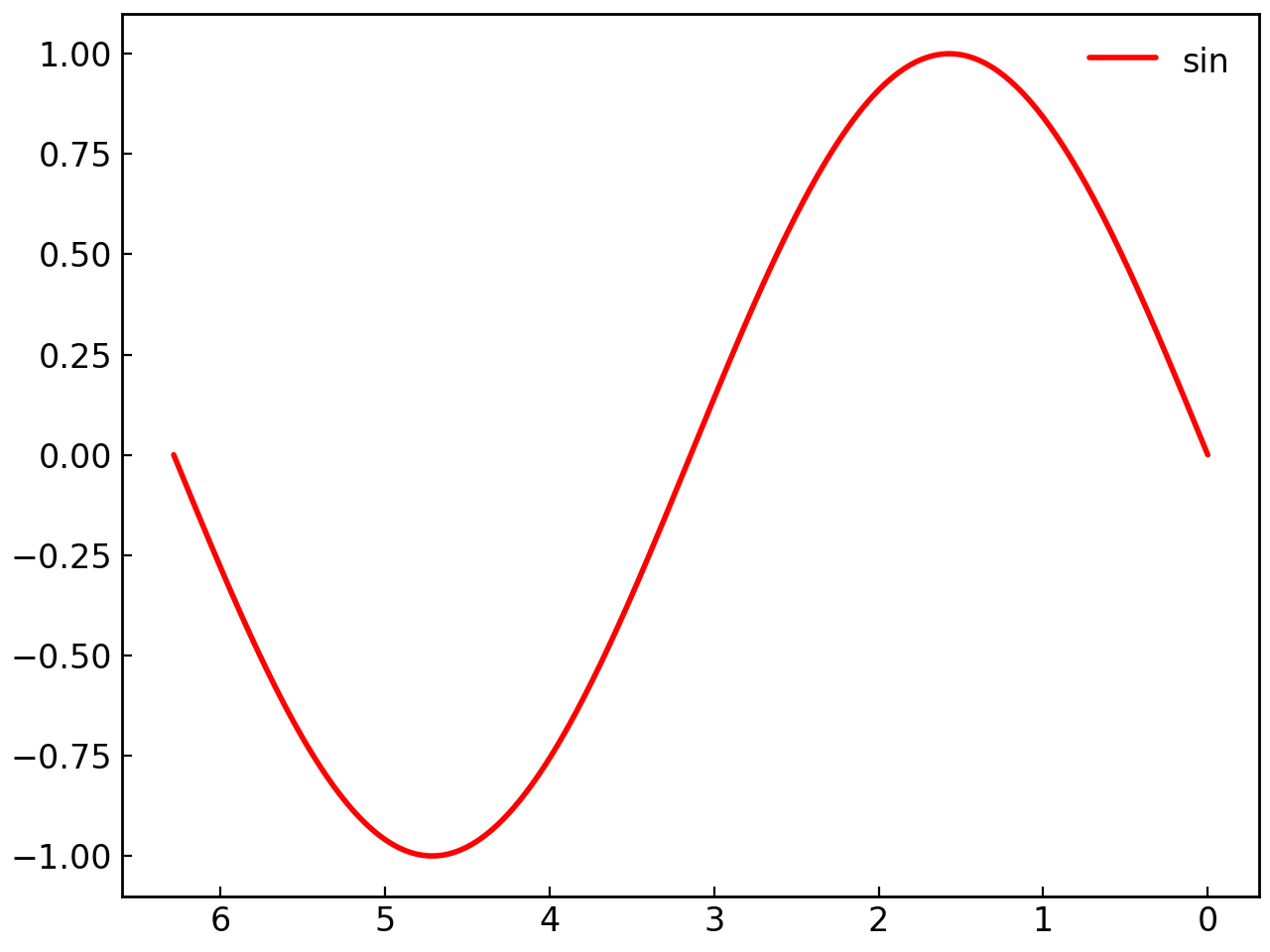
fig = gl.SmartFigure(
    invert_x_axis=True,
    invert_y_axis=False,
    elements=curve1,
)
fig.show()

(png, hires.png, pdf)

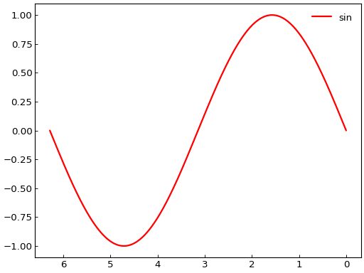
Note

This can also be done by inverting directly the axes’ limits with x_lim and y_lim parameters (e.g. x_lim=(max, min)).

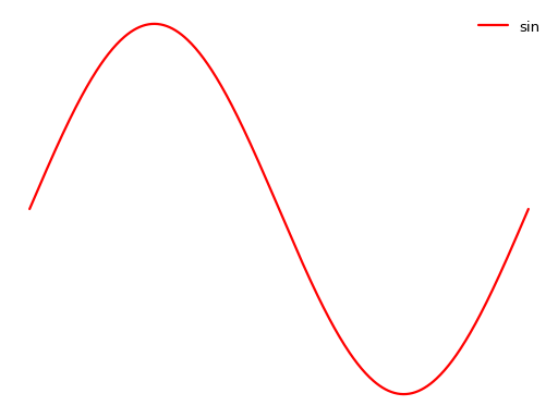
Removing Axes and Ticks

# Remove entire axes
fig = gl.SmartFigure(
    remove_axes=True,
    elements=curve1,
)
fig.show()

(png, hires.png, pdf)

# Remove only ticks
fig = gl.SmartFigure(
    remove_x_ticks=True,
    remove_y_ticks=False,
    elements=curve1,
)
fig.show()

(png, hires.png, pdf)

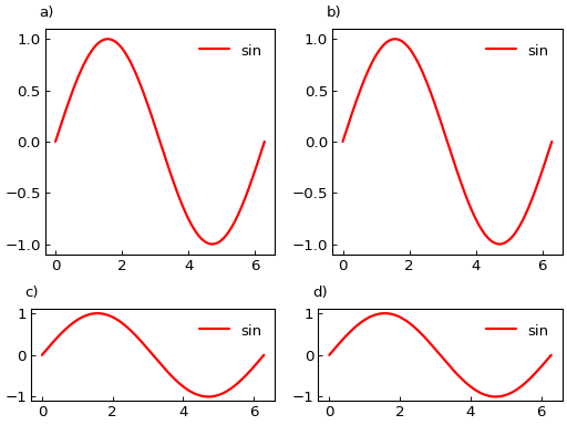
Sharing Axes

Share axes between subplots for synchronized zooming and consistent limits:

fig = gl.SmartFigure(
    2, 2,
    share_x=True,
    share_y=True,
    elements=[curve1, curve2, curve1, curve2]
)
fig.show()

(png, hires.png, pdf)

Note

Axis sharing affects the plots drawn directly in the parent layout. If you insert an existing nested SmartFigure, that nested figure controls its own axis sharing independently.

Warning

The SmartFigure is currently testing an experimental method for perfectly aligning horizontally shared subplots when share_x=True. This may not work in all cases and could be subject to change in future versions. If you encounter issues, please report them on the GraphingLib GitHub issue tracker.

Advanced Customization Methods

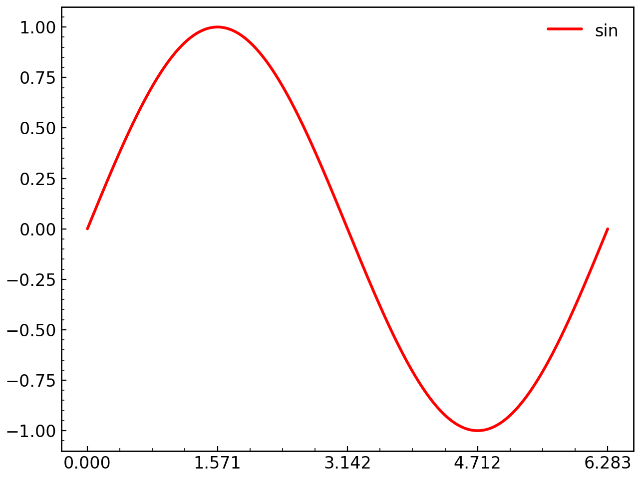
Custom Ticks

The set_ticks() method provides fine-grained control over tick positions and labels:

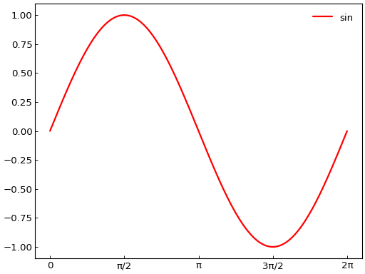
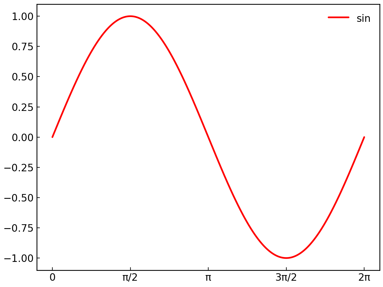
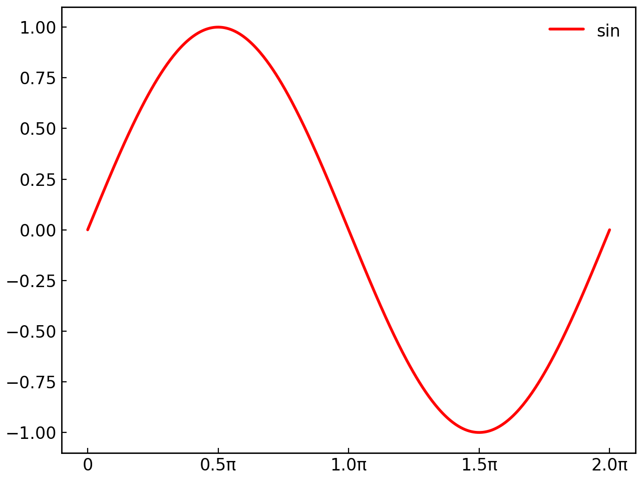
fig = gl.SmartFigure(elements=curve1)

# Set custom tick positions
fig.set_ticks(
    x_ticks=[0, np.pi/2, np.pi, 3*np.pi/2, 2*np.pi],
    x_tick_labels=["0", "π/2", "π", "3π/2", "2π"]
)
fig.show()

(png, hires.png, pdf)

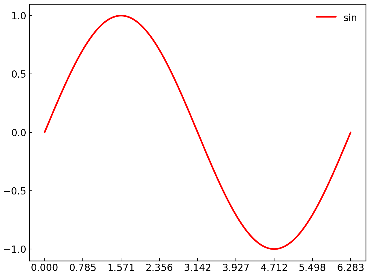
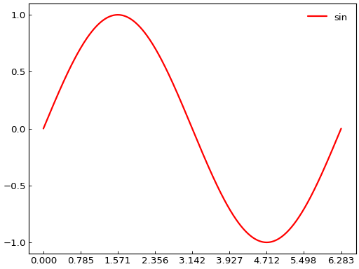
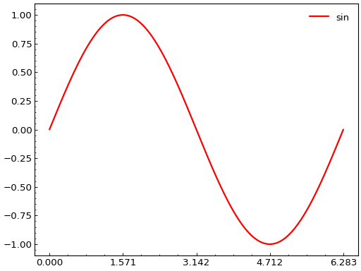
# Use automatic spacing
fig = gl.SmartFigure(elements=curve1)
fig.set_ticks(
    x_tick_spacing=np.pi/4,
    y_tick_spacing=0.5
)
fig.show()

(png, hires.png, pdf)

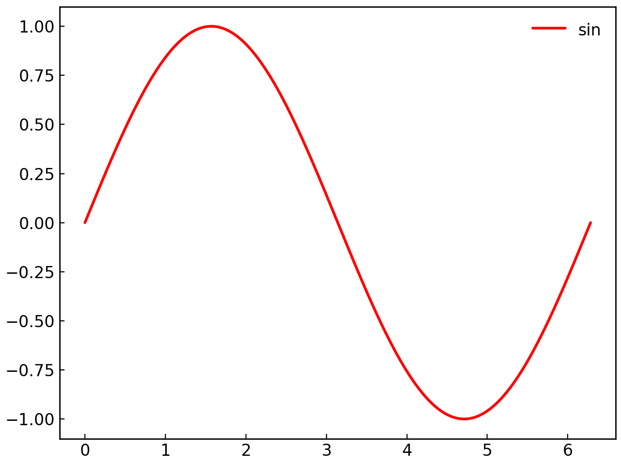
# Add minor ticks
fig = gl.SmartFigure(elements=curve1)
fig.set_ticks(
    x_tick_spacing=np.pi/2,
    minor_x_tick_spacing=np.pi/8,
    minor_y_tick_spacing=0.05
)
fig.show()

(png, hires.png, pdf)

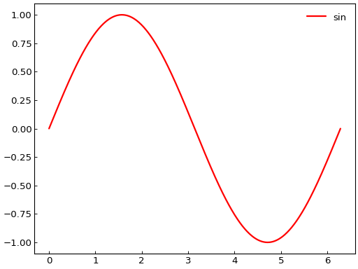
# Reset to defaults
fig = gl.SmartFigure(elements=curve1)
fig.set_ticks(x_tick_spacing=1.0)  # Set custom ticks
fig.set_ticks(reset=True)  # Reset to default behavior
fig.show()

(png, hires.png, pdf)

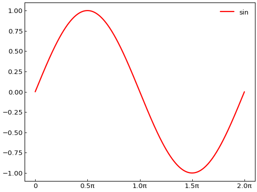
You can also provide a custom tick label formatter function that takes a tick value and returns a string label:

# Use a formatter and specify tick positions
formatter = lambda v: f"{v/np.pi:.1f}π" if v != 0 else "0"

fig = gl.SmartFigure(elements=curve1)
fig.set_ticks(
    x_ticks=[0, np.pi/2, np.pi, 3*np.pi/2, 2*np.pi],
    x_tick_labels=formatter
)
fig.show()

(png, hires.png, pdf)

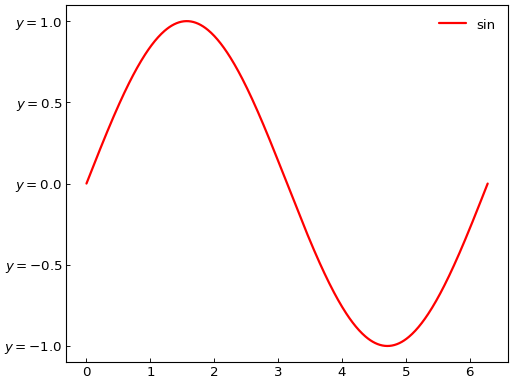
# Use a formatter and specify tick spacing
formatter = lambda v: f"$y={v}$"

fig = gl.SmartFigure(elements=curve1)
fig.set_ticks(
    y_tick_spacing=0.5,
    y_tick_labels=formatter,
)
fig.show()

(png, hires.png, pdf)

Warning

Since tick position and tick spacing are conflicting parameters, trying to set both at the same time for the same axis will raise an error. Similarly, giving tick labels as a list without giving tick positions will also raise an error. For more details on the possible combinations of parameters, see the set_ticks() method docstring.

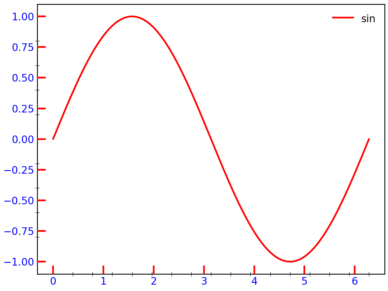
Tick Appearance

The set_tick_params() method controls tick appearance. You can also give parameters separately for major and minor ticks as well as for each axis:

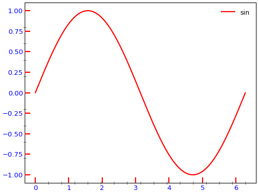
fig = gl.SmartFigure(elements=curve1)

# Customize major ticks
fig.set_tick_params(
    axis="both",
    which="major",
    direction="in",
    length=10,
    width=2,
    color="red",
    label_size=12,
    label_color="blue"
)

# Customize minor ticks
fig.set_tick_params(
    axis="both",
    which="minor",
    direction="inout",
    length=5,
    width=0.5
)
fig.set_ticks(minor_x_tick_spacing=np.pi/8, minor_y_tick_spacing=0.2)

fig.show()

(png, hires.png, pdf)

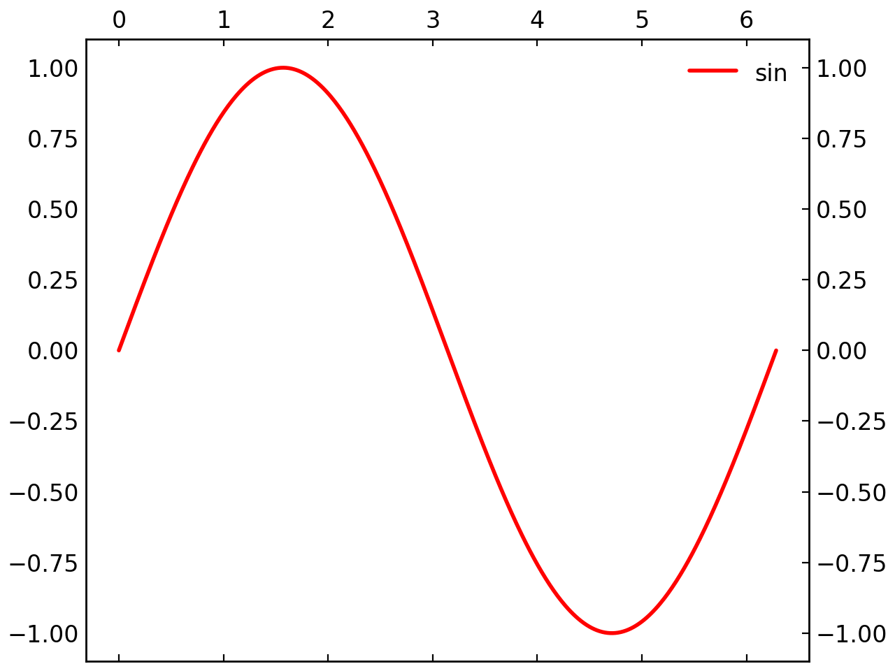
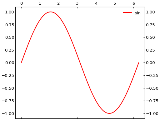
You can also control the presence of ticks and labels on specific sides of the plot:

fig = gl.SmartFigure(elements=curve1)
fig.set_tick_params(
    axis="x",
    draw_top_ticks=True,
    draw_top_labels=True,
    draw_bottom_labels=False
)
fig.set_tick_params(
    axis="y",
    draw_right_ticks=True,
    draw_right_labels=True,
    draw_left_ticks=False,
)
fig.show()

(png, hires.png, pdf)

Grid Customization

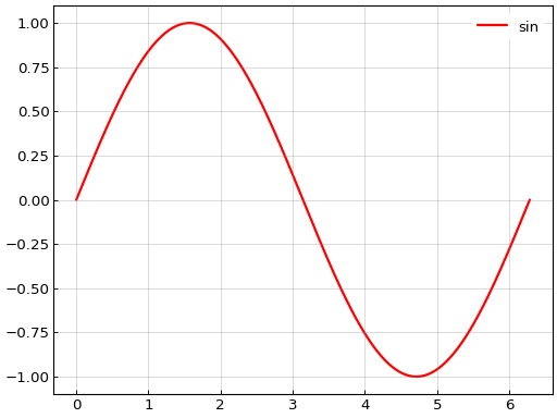
The set_grid() method enables and customizes grid lines:

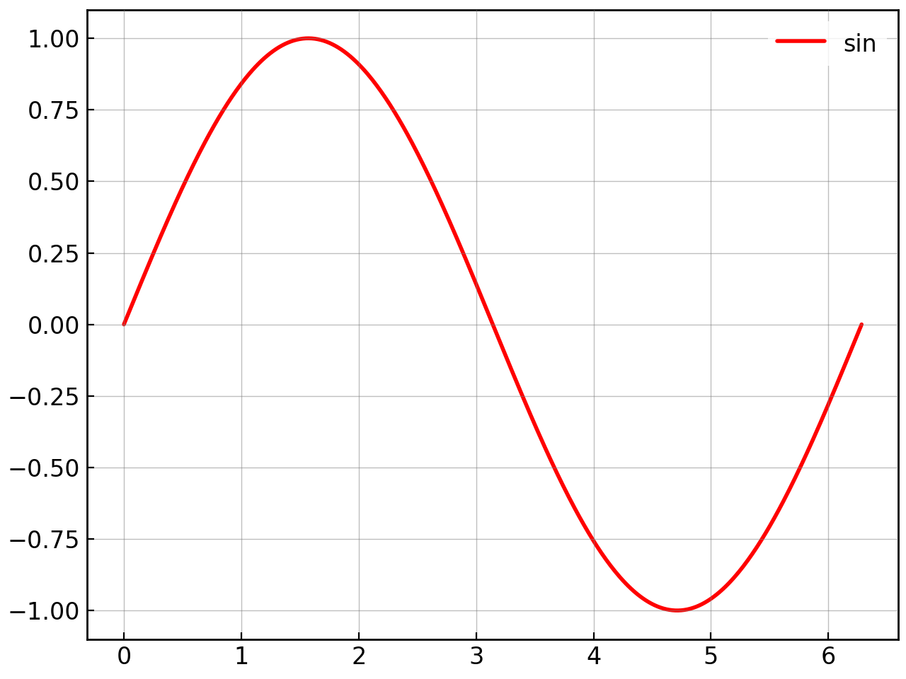
fig = gl.SmartFigure(elements=curve1)

# Basic grid
fig.set_grid()
fig.show()

(png, hires.png, pdf)

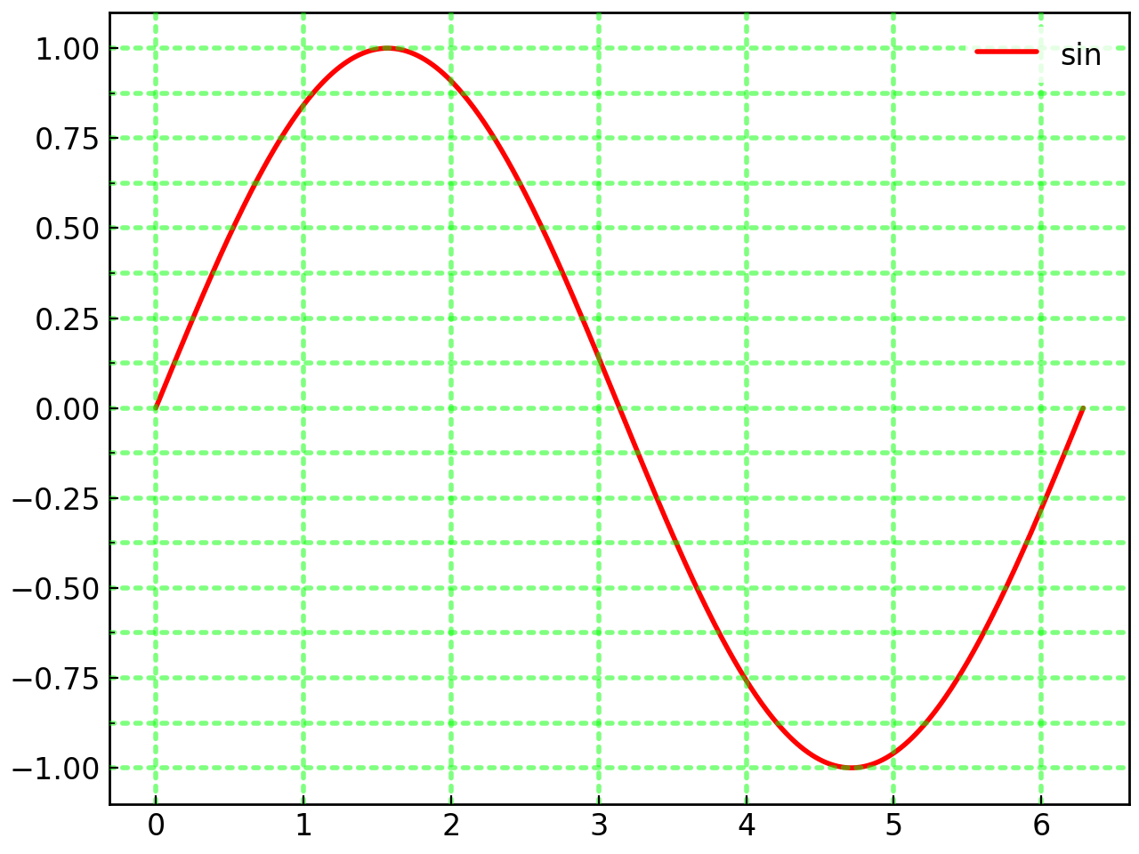
The same parameters are applied to both axes and major and minor grid lines, but you can control their visibility separately:

# Customize grid appearance
fig = gl.SmartFigure(elements=curve1)
fig.set_grid(
    visible_x=True,
    visible_y=True,
    which_x="major",  # Only major gridlines on x
    which_y="both",   # Both major and minor on y
    color="lime",
    alpha=0.5,
    line_style=":",
    line_width=2
)
# Need minor ticks for minor gridlines
fig.set_ticks(minor_y_tick_spacing=0.125)
fig.show()

(png, hires.png, pdf)

Note

Once you have enabled the grid with set_grid(), you can toggle its visibility using the show_grid property.

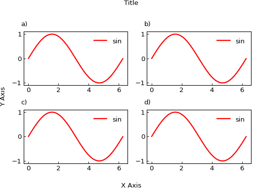
Text Padding

The set_text_padding_params() method controls spacing around text elements:

fig = gl.SmartFigure(
    2, 2,
    x_label="X Axis",
    y_label="Y Axis",
    title="Title",
    elements=[curve1]*4
)

# Increase padding
fig.set_text_padding_params(
    x_label_pad=20,
    y_label_pad=10,
    title_pad=30
)
fig.show()

(png, hires.png, pdf)

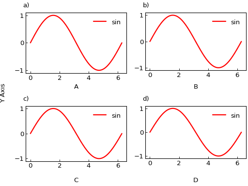
If you are using sub_x_labels, sub_y_labels, or subtitles, you can also control their padding independently:

fig = gl.SmartFigure(
    2, 2,
    y_label="Y Axis",
    sub_x_labels=["A", "B", "C", "D"],
    elements=[curve1]*4
)
fig.set_text_padding_params(
    sub_x_labels_pad=[5, 10, 15, 20],  # Different padding for each
    y_label_pad=15
)
fig.show()

(png, hires.png, pdf)

Annotations

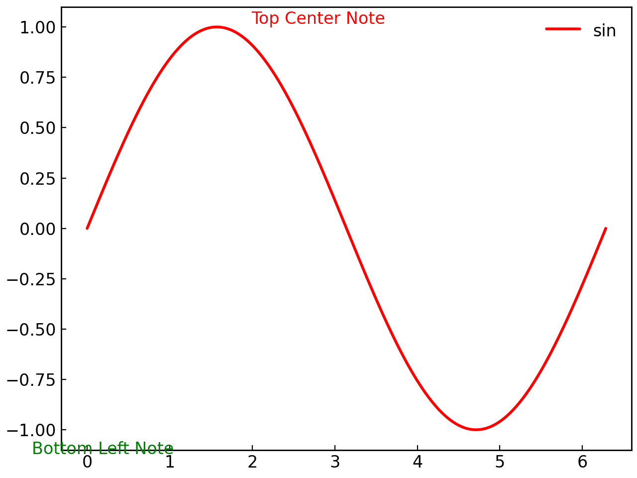
Other than adding Text elements directly to subplots, you can also add annotations to the figure as a whole using the annotations parameter:

# Create annotations (coordinates in range [0, 1])
note1 = gl.Text(0.5, 0.95, "Top Center Note", "red", h_align="center")
note2 = gl.Text(0.05, 0.05, "Bottom Left Note", "green")

fig = gl.SmartFigure(
    elements=curve1,
    annotations=[note1, note2]
)
fig.show()

(png, hires.png, pdf)

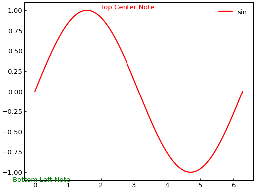
Note

Annotations use figure-relative coordinates, not data coordinates. This makes them useful for notes that should appear in fixed positions regardless of data scales. This also allows them to be placed outside the axes area.

Properties That Accept Lists or Single Items

Many properties of the SmartFigure class are typed as ListOrItem, a flexible type that allows you to provide either a single value or a list of values. This feature is essential for customizing figures where different subfigures may need different configurations.

Understanding the ListOrItem Type

The ListOrItem type is a type hint defined as:

ListOrItem = Union[T, list[T]]

where T is any type. This means that any property documented as ListOrItem[float] (for example) can accept either a single float value or a list[float].

When you provide a single value, it is applied to all subfigures drawn by the SmartFigure. When you provide a list of values, each value is applied to the corresponding subfigure from left to right, top to bottom.

List Length and Padding Rules

When using lists with SmartFigure, the following rules apply to list length:

Shorter than number of subfigures drawn by the SmartFigure:

The list is padded with the default value for that property. For example, if you have 4 subfigures but only provide 2 values in a list, the remaining 2 subfigures will use the default value.

Equal to number of subfigures drawn by the SmartFigure:

Perfect! Each value maps exactly to one subfigure.

Longer than number of subfigures drawn by the SmartFigure:

An error is raised. The list cannot have more values than there are subfigures.

Special case - Nested SmartFigures:

When a subfigure contains a nested SmartFigure, that nested figure still counts as one entry in the list mapping. Likewise, a child SmartFigure spanning multiple cells still counts as one entry. As such, you may need to pad your lists with any value to account for nested figures which control their own properties and will ignore this parameter.

Note

The number of subfigures drawn by the SmartFigure corresponds to the number of child plots or nested figures that will actually be drawn. This excludes positions set to None but includes positions that are drawn but empty (for example, set to []). Subfigures that span multiple rows or columns are also counted as one subfigure. For a SmartFigure used as a layout, the __len__() method returns this number. For a SmartFigure used as a single plot, __len__() instead returns the number of plotted elements in that plot.

Properties That Accept ListOrItem

The following properties accept ListOrItem values:

Property	Type	Default Value
x_lim	ListOrItem[tuple[float, float] | None]	None
y_lim	ListOrItem[tuple[float, float] | None]	None
log_scale_x	ListOrItem[bool]	False
log_scale_y	ListOrItem[bool]	False
remove_axes	ListOrItem[bool]	False
aspect_ratio	ListOrItem[float | Literal["auto", "equal"]]	"auto"
box_aspect_ratio	ListOrItem[float | None]	None
remove_x_ticks	ListOrItem[bool]	False
remove_y_ticks	ListOrItem[bool]	False
invert_x_axis	ListOrItem[bool]	False
invert_y_axis	ListOrItem[bool]	False
reference_labels	ListOrItem[bool]	True
reference_labels_loc	ListOrItem[Literal["inside", "outside"] | tuple[float, float]]	"outside"
projection	ListOrItem[Any | None]	None
legend_loc	ListOrItem[str | tuple | None]	None
legend_cols	ListOrItem[int]	1
show_legend	ListOrItem[bool]	True
show_grid	ListOrItem[bool]	False
hide_default_legend_elements	ListOrItem[bool]	False

Warning

When general_legend is set to True, legend properties must be provided as single values and cannot be lists, since there is only one legend for the entire figure. If a list is provided, an error will be raised during figure creation. Parameters affected are legend_loc, legend_cols, show_legend and hide_default_legend_elements. Note that the hide_custom_legend_elements parameter must always be a single value since it applies to the entire figure.

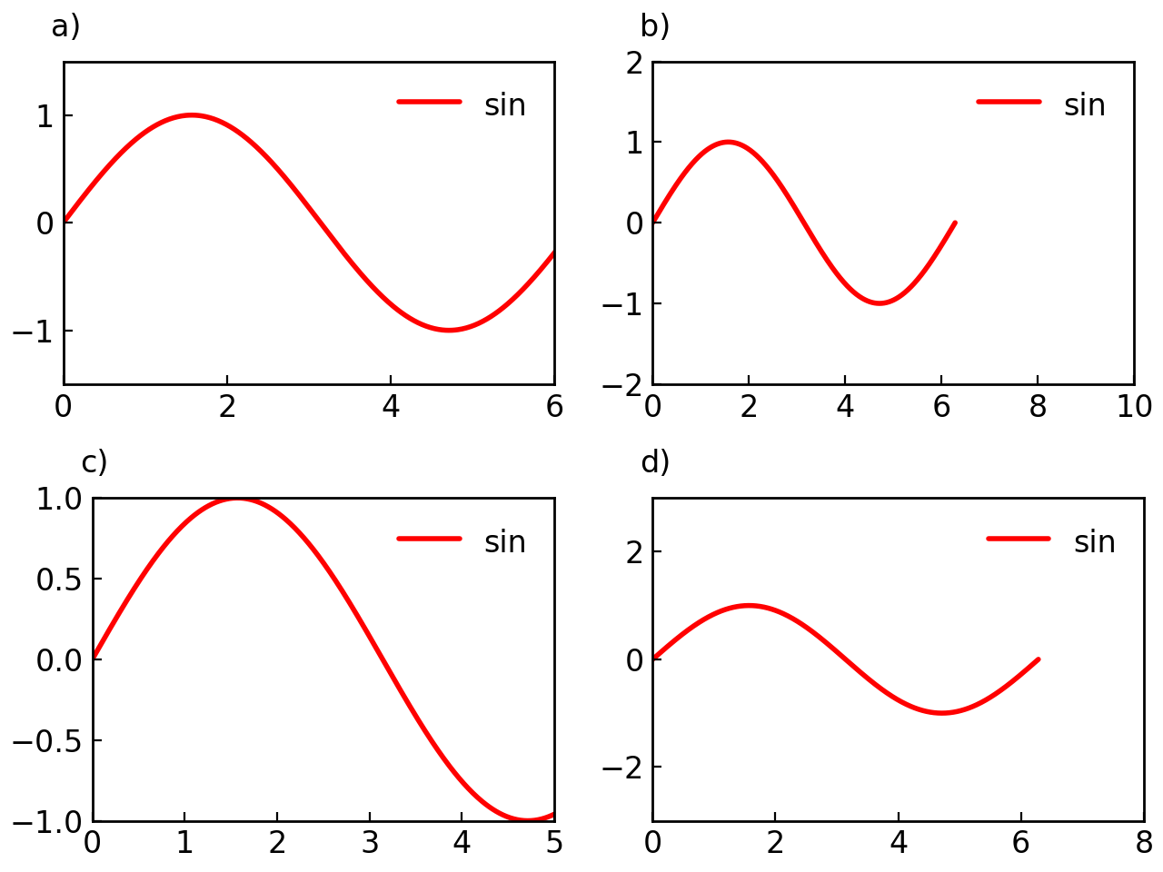
Examples of Using Lists

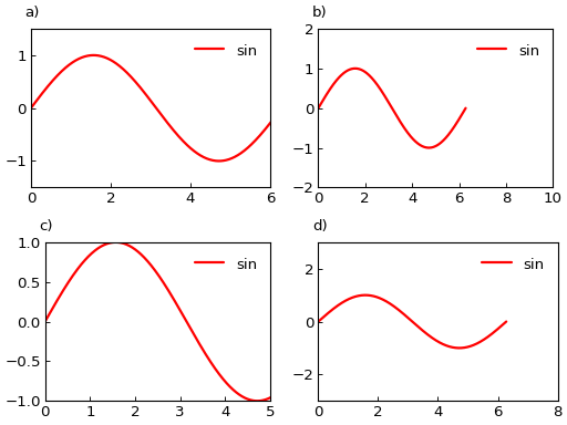
Here are practical examples showing how to use lists with these properties:

# List of values - each subplot gets different limits
fig = gl.SmartFigure(
    2, 2,
    x_lim=[(0, 6), (0, 10), (0, 5), (0, 8)],  # Different x limits per subplot
    y_lim=[(-1.5, 1.5), (-2, 2), (-1, 1), (-3, 3)],  # Different y limits per subplot
    elements=[curve1]*4
)
fig.show()

(png, hires.png, pdf)

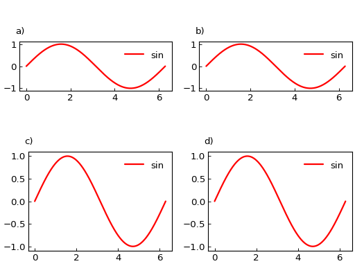
# Shortened list - padded with defaults
fig = gl.SmartFigure(
    2, 2,
    aspect_ratio=["equal", "equal"],  # Only first 2 subplots get equal aspect ratio
    # Remaining 2 subplots use the default "auto"
    elements=[curve1]*4
)
fig.show()

(png, hires.png, pdf)

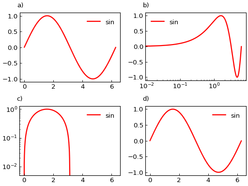
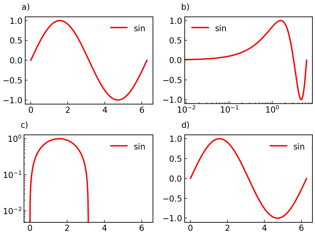
# Different log scales per subplot
fig = gl.SmartFigure(
    2, 2,
    log_scale_x=[False, True, False],  # Last subplot uses default False
    log_scale_y=[False, False, True, False],
    elements=[curve1]*4
)
fig.show()

(png, hires.png, pdf)

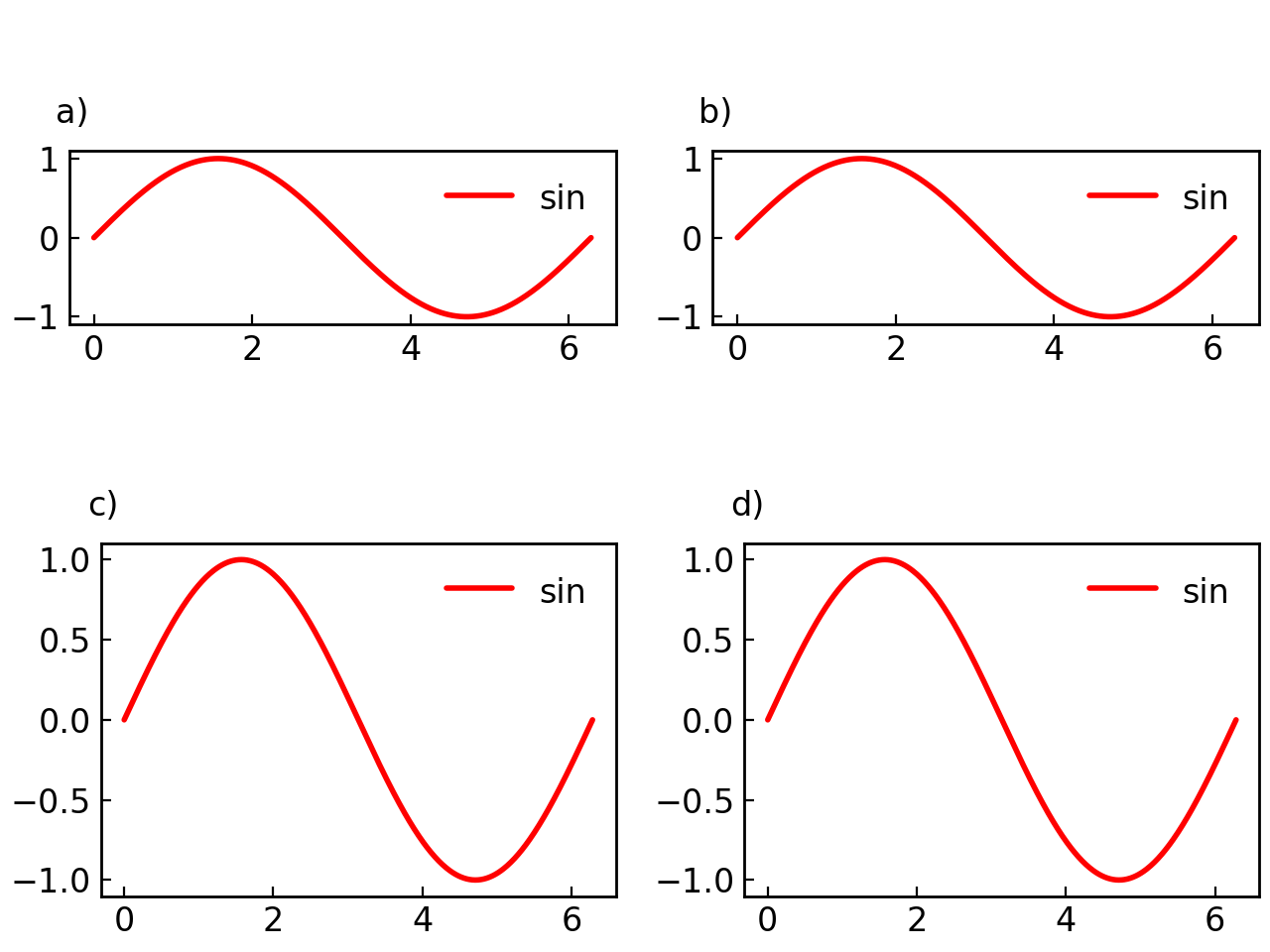
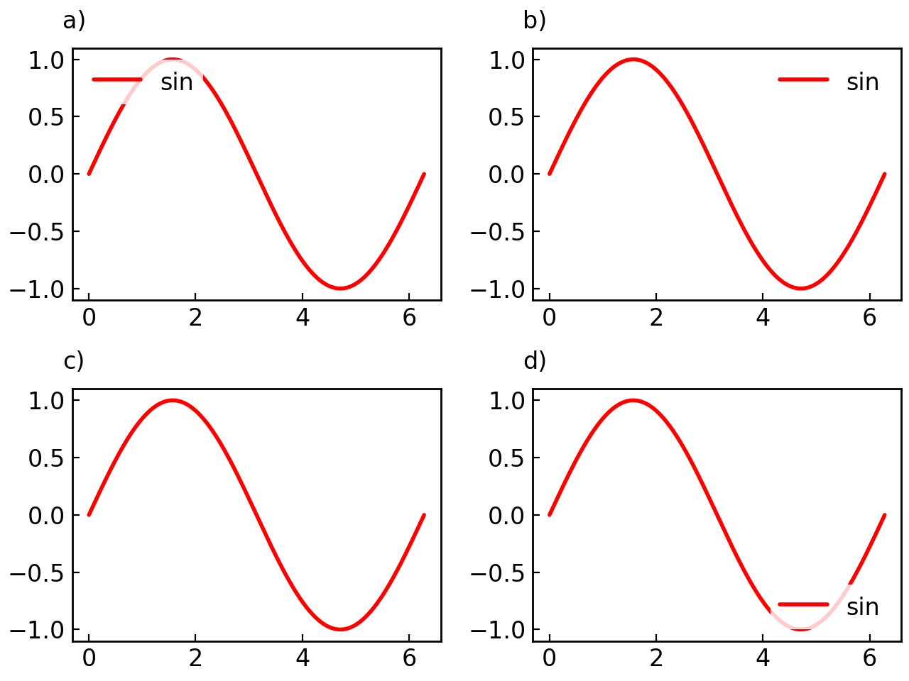
# Different legend configurations per subplot
fig = gl.SmartFigure(
    2, 2,
    legend_loc=["upper left", "upper right", "lower left", "lower right"],
    show_legend=[True, True, False, True],  # Hide legend in third subplot
    elements=[curve1]*4
)
fig.show()

(png, hires.png, pdf)

Visual Styling

Figure Styles

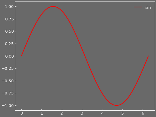
The figure_style parameter applies predefined visual themes:

# GraphingLib built-in styles
fig = gl.SmartFigure(
    figure_style="dim",
    elements=curve1,
)
fig.show()

(png, hires.png, pdf)

# Matplotlib styles
fig = gl.SmartFigure(
    figure_style="seaborn-v0_8",
    elements=curve1,
)
fig.show()

(png, hires.png, pdf)

See also

See Writing your own figure style file for creating custom styles.

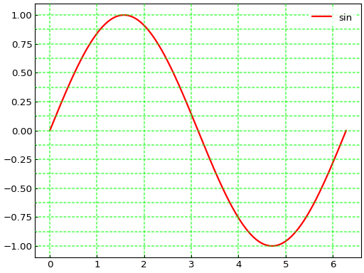
RC Parameters Method

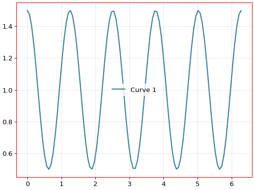
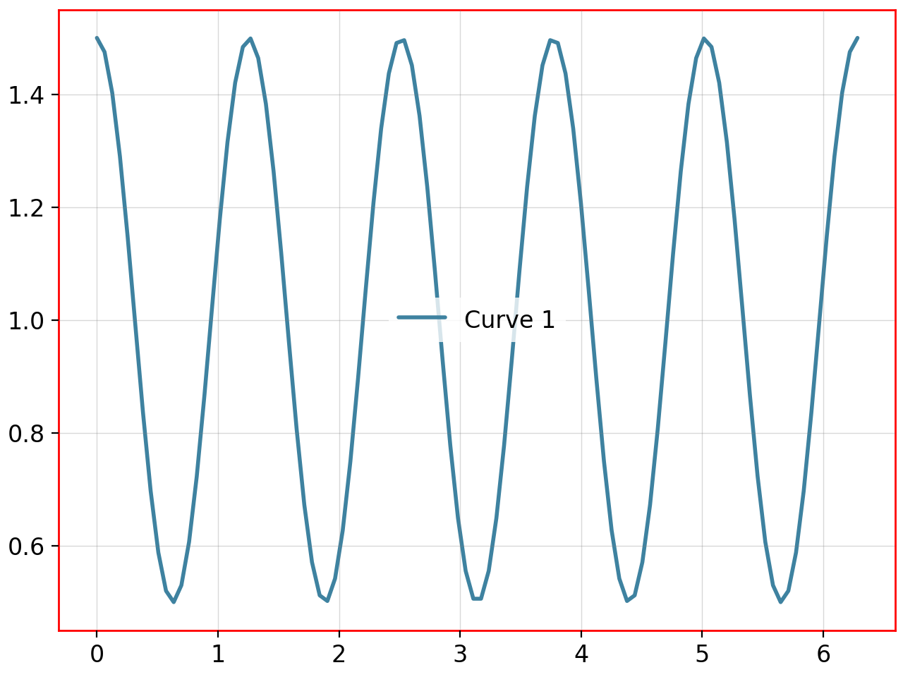
The set_rc_params() method provides direct access to matplotlib’s rcParams:

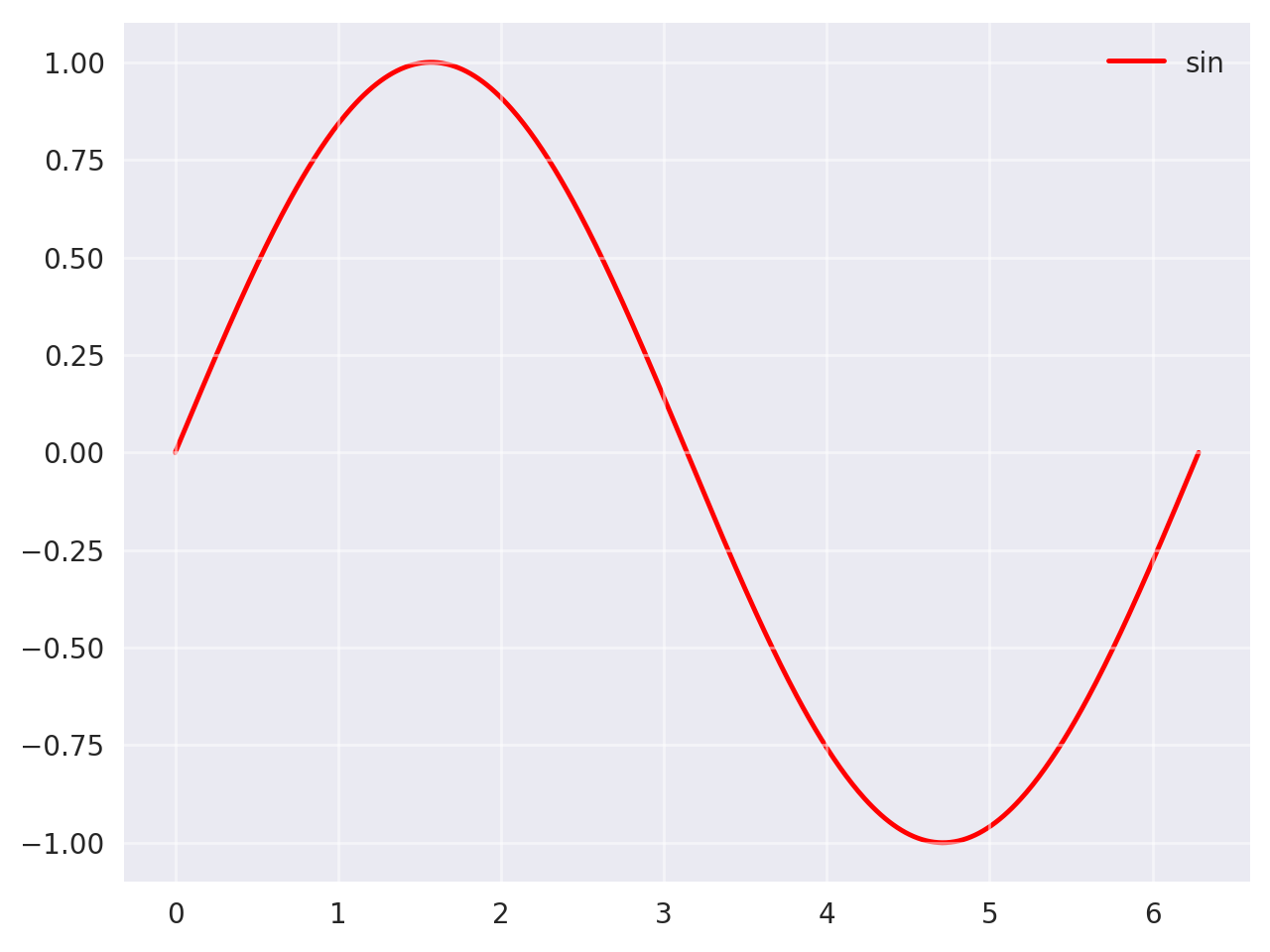
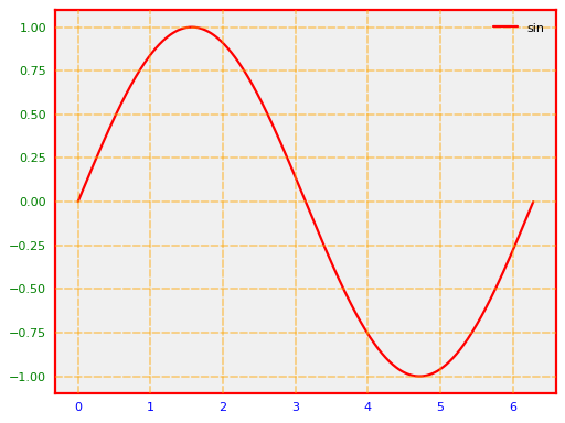
fig = gl.SmartFigure(elements=curve1)

fig.set_rc_params({
    "axes.facecolor": "#f0f0f0",
    "axes.edgecolor": "red",
    "axes.linewidth": 2,
    "xtick.color": "blue",
    "ytick.color": "green",
    "grid.color": "orange",
    "grid.linestyle": "--",
    "grid.linewidth": 1.5
})
fig.set_grid()

fig.show()

(png, hires.png, pdf)

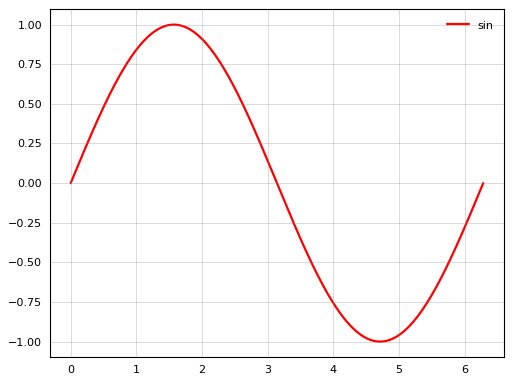
# Reset parameters
fig.set_rc_params(reset=True)
fig.show()

(png, hires.png, pdf)

Visual Parameters Method

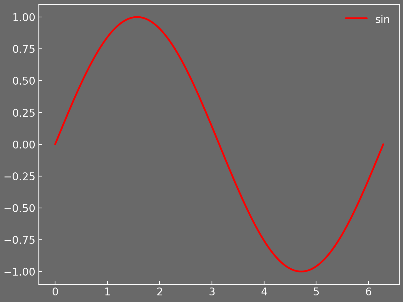
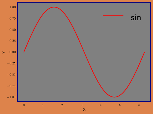
The set_visual_params() method provides a convenient interface for common styling:

fig = gl.SmartFigure(
    x_label="X",
    y_label="Y",
    elements=curve1,
)

fig.set_visual_params(
    figure_face_color="#dd834bff",
    axes_face_color="grey",
    axes_edge_color="navy",
    axes_line_width=2,
    legend_font_size=30,
    use_latex=True
)

fig.show()

(png, hires.png, pdf)

# Color cycle for multiple elements
fig = gl.SmartFigure(elements=[curve1, curve2])
fig.set_visual_params(
    color_cycle=["#FF6B6B", "#4ECDC4", "#45B7D1"]
)
fig.show()

(png, hires.png, pdf)

# Hide individual spines
fig = gl.SmartFigure(elements=curve1)
fig.set_visual_params(
    hidden_spines=["top", "right"]
)
fig.show()

(png, hires.png, pdf)

Legend Control

Legend customization has many options:

Basic Legend Control

# Control legend visibility
fig = gl.SmartFigure(
    show_legend=False,  # Hide legend
    elements=[curve1, curve2]
)
fig.show()

(png, hires.png, pdf)

# Legend location
fig = gl.SmartFigure(
    legend_loc="lower left",
    elements=[curve1, curve2]
)
fig.show()

(png, hires.png, pdf)

# Multi-column legend
fig = gl.SmartFigure(
    legend_cols=2,
    elements=[curve1, curve2]
)
fig.show()

(png, hires.png, pdf)

General Legend

For multi-subplot figures, create a single legend for all subplots:

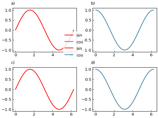
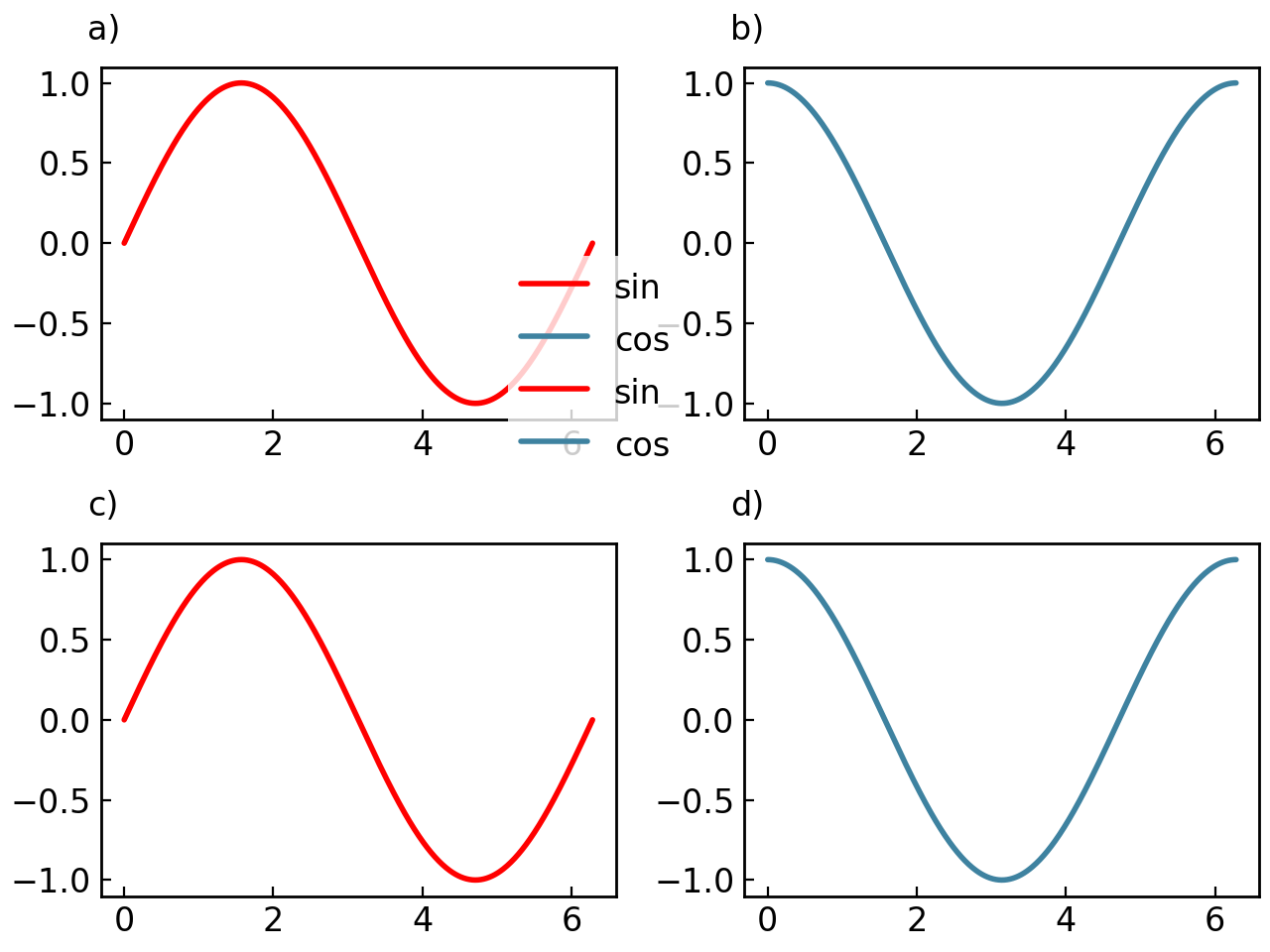
fig = gl.SmartFigure(
    2, 2,
    general_legend=True,
    legend_loc=(0.4, 0.5),
    elements=[curve1, curve2, curve1, curve2]
)
fig.show()

(png, hires.png, pdf)

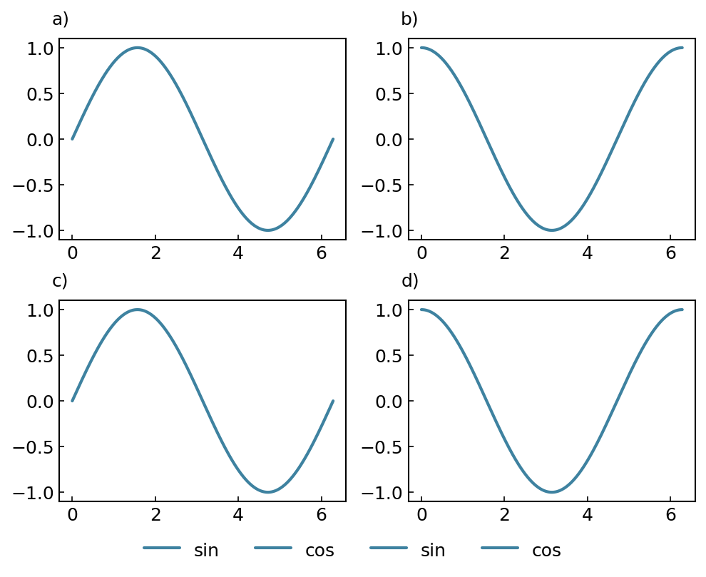
# Outside legend positions
fig = gl.SmartFigure(
    2, 2,
    general_legend=True,
    legend_loc="outside lower center",
    legend_cols=4,
    elements=[curve1, curve2, curve1, curve2]
)
fig.save("output.png")  # Or use inline Jupyter display

Warning

General legends with a location beginning with "outside" may not be displayed correctly since matplotlib does not change the window size to accomodate for the legend position. In such cases, use inline Jupyter display or save the figure to a file to see the legend on the figure.

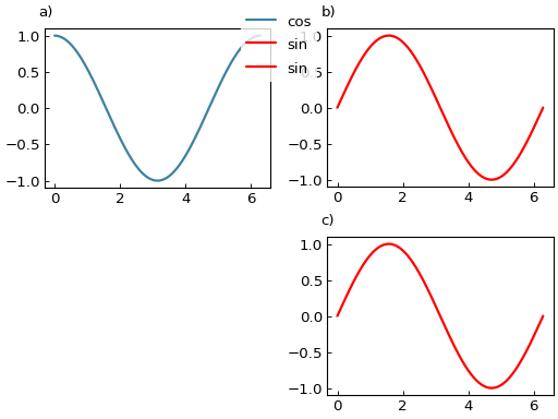
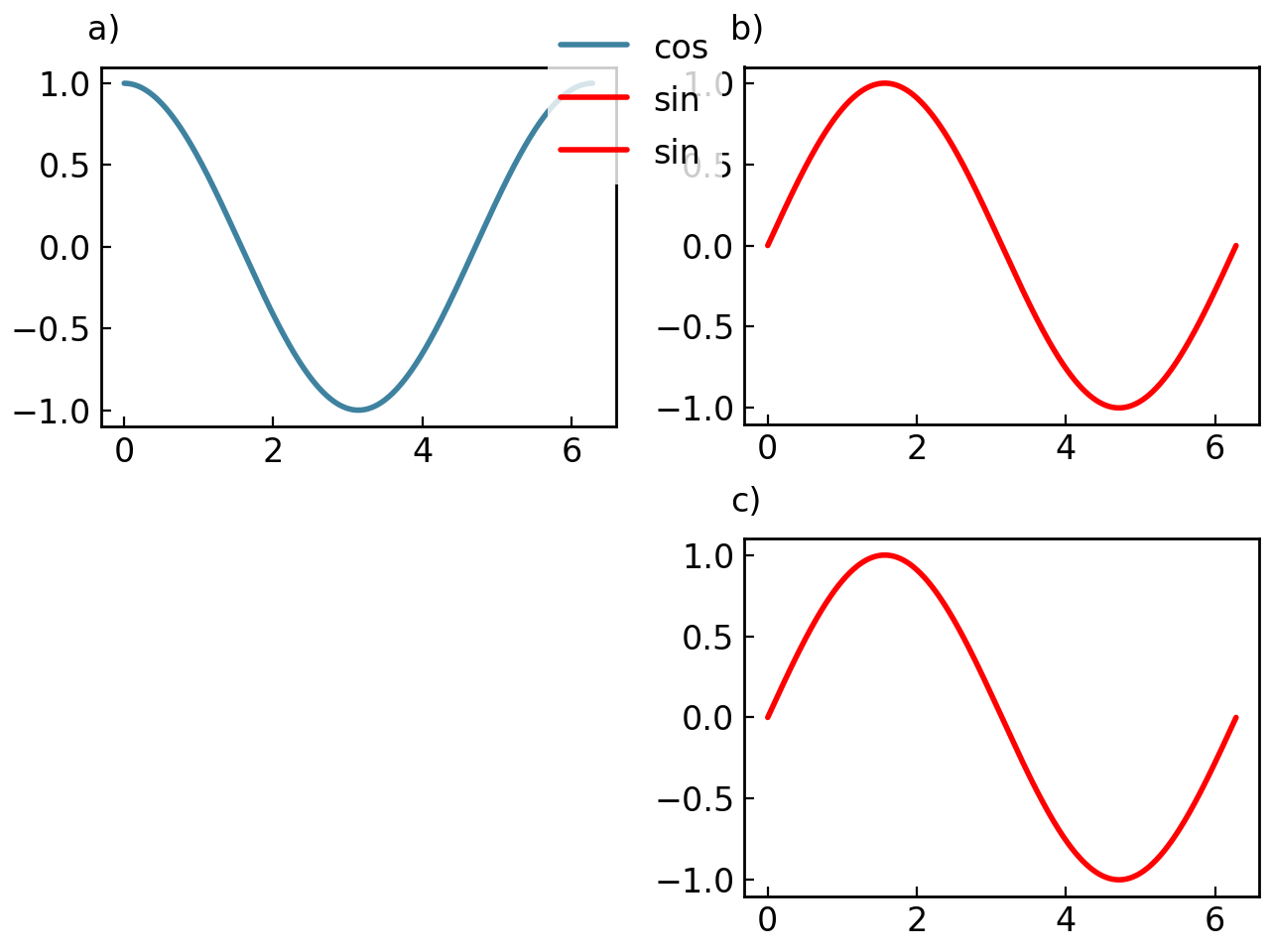
If you have a nested SmartFigure, you can create a general legend for the entire figure including all sub-figures:

# Create individual figures
fig1 = gl.SmartFigure(2, 1, elements=[curve1, curve1])
fig2 = gl.SmartFigure(num_rows=2, num_cols=2, general_legend=True, legend_loc="upper center")
fig2[0, 0] = curve2
fig2[:, 1] = fig1
fig2.show()

(png, hires.png, pdf)

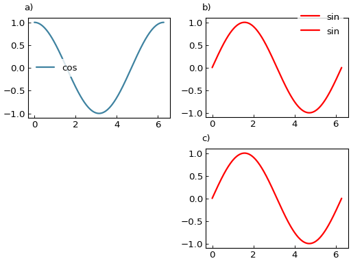
You can alternatively choose that each nested figure creates its own general legend, in which case you need to specify general_legend=True for that nested SmartFigure:

# Create individual figures
fig1 = gl.SmartFigure(
    2, 1,
    general_legend=True,
    legend_loc="upper right",
    elements=[curve1, curve1]
)
fig2 = gl.SmartFigure(num_rows=2, num_cols=2, legend_loc="center left")
fig2[0, 0] = curve2
fig2[:, 1] = fig1

fig2.show()

(png, hires.png, pdf)

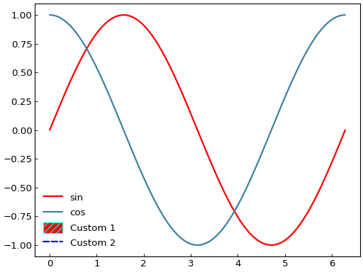
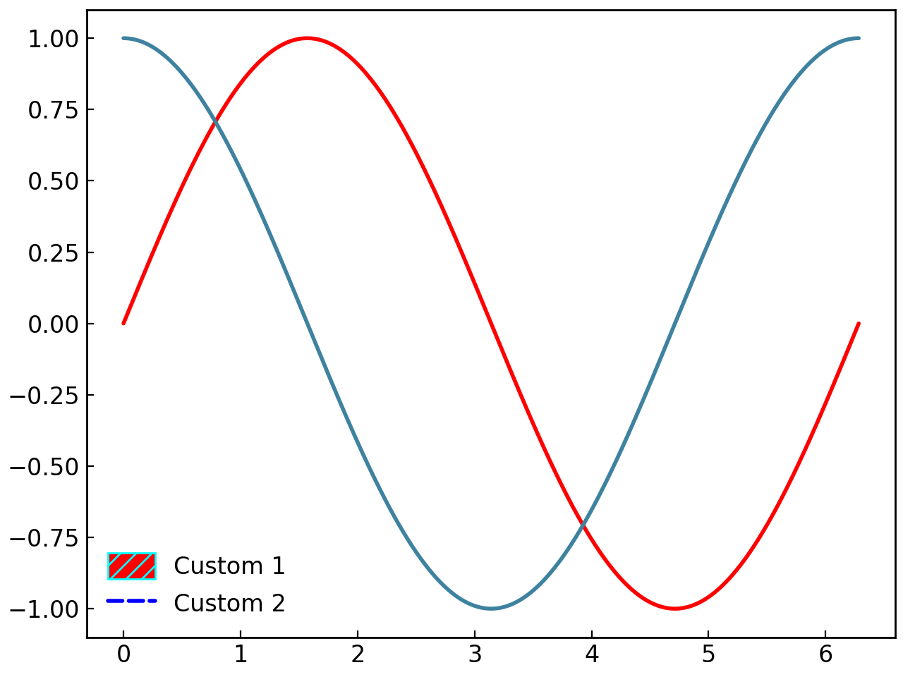
Custom Legend Elements

The set_custom_legend() method adds custom legend entries:

# Create custom legend elements
custom_elem1 = gl.LegendPatch("Custom 1", "red", "cyan", hatch="///")
custom_elem2 = gl.LegendLine("Custom 2", "blue", line_style="dashed")

fig = gl.SmartFigure(elements=[curve1, curve2])
fig.set_custom_legend(elements=[custom_elem1, custom_elem2])
fig.show()

(png, hires.png, pdf)

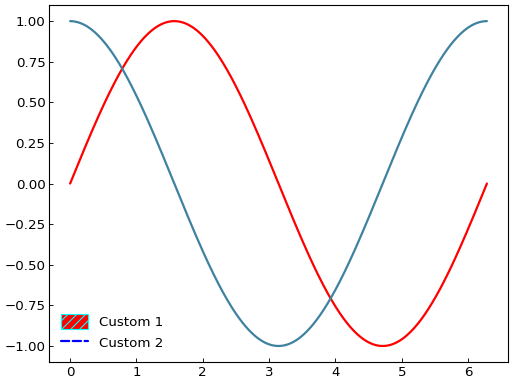
# Hide default elements, show only custom
fig.hide_default_legend_elements = True
fig.show()

(png, hires.png, pdf)

# Hide custom elements, show only default
fig.hide_default_legend_elements = False
fig.hide_custom_legend_elements = True
fig.show()

(png, hires.png, pdf)

See also

See the LegendLine, LegendMarker, and LegendPatch classes for creating custom legend elements.

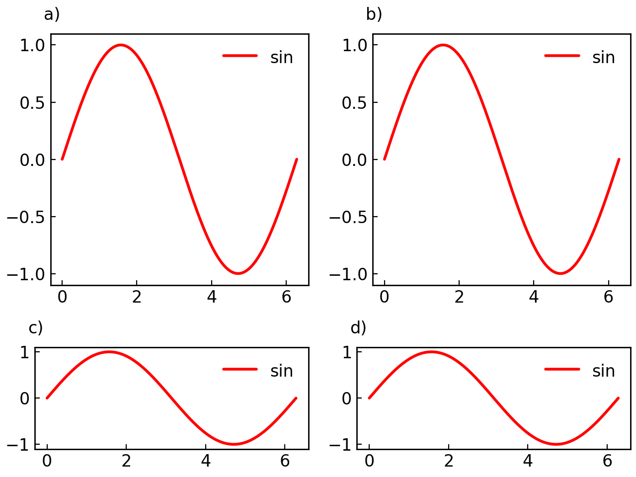
Reference Labels

Reference labels (a), b), c), etc.) help identify subplots in publications:

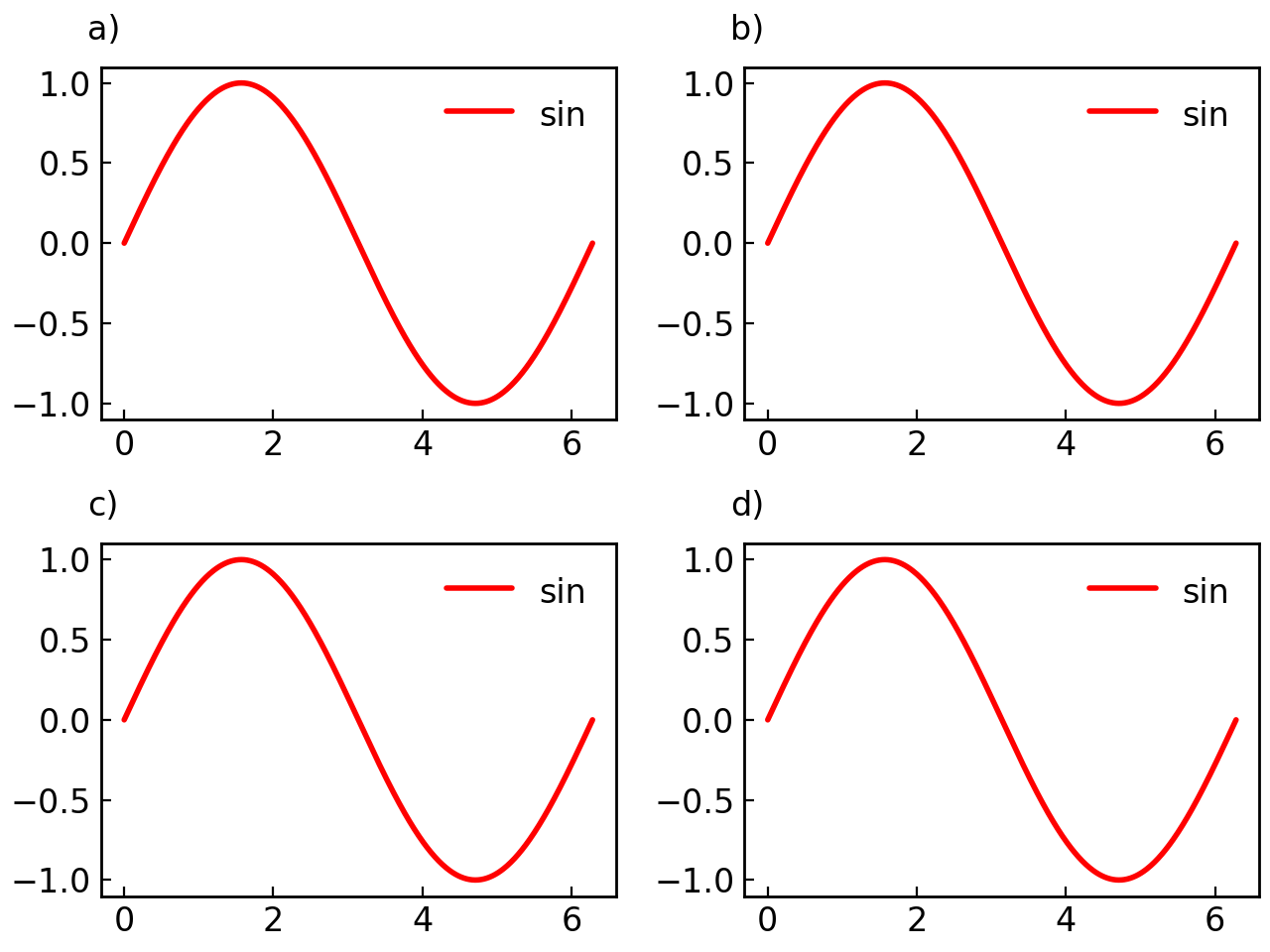
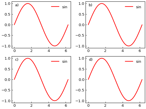
Basic Reference Labels

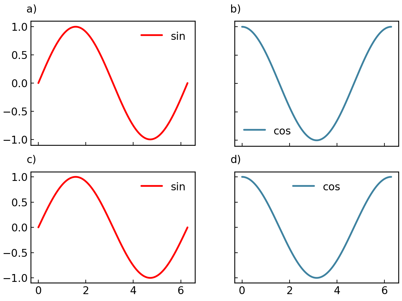
Reference labels are enabled by default:

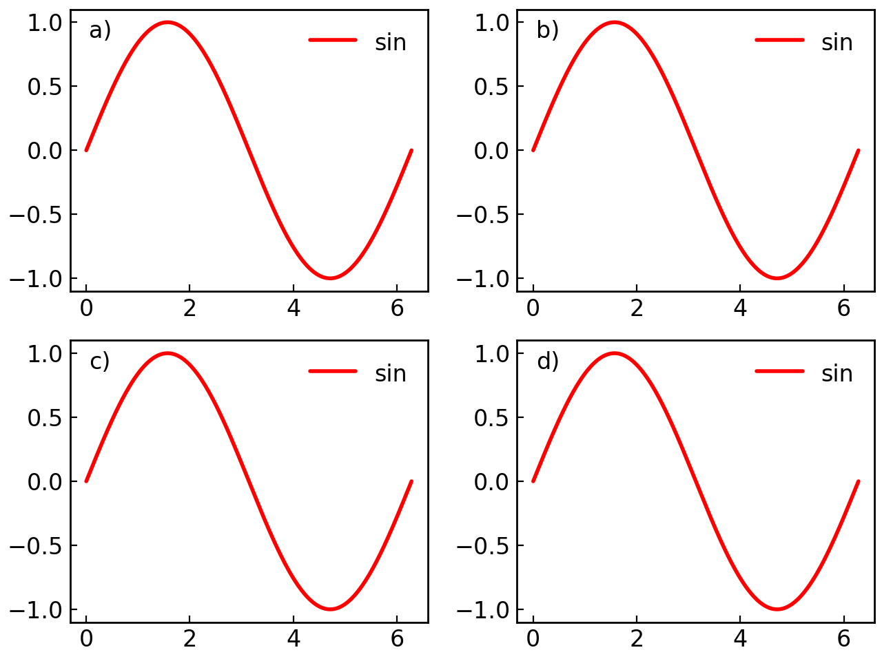
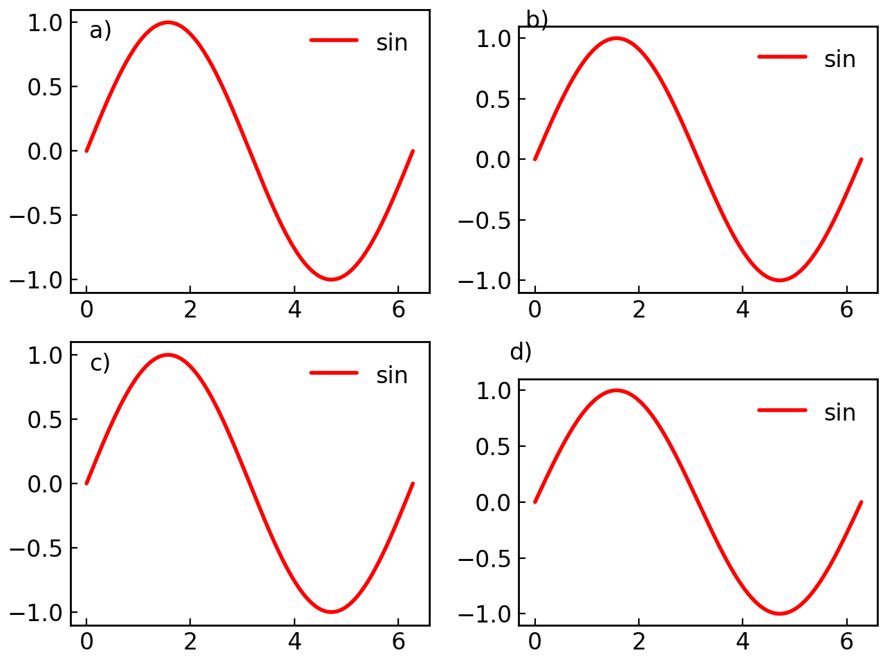
fig = gl.SmartFigure(2, 2, elements=[curve1]*4)
fig.show()

(png, hires.png, pdf)

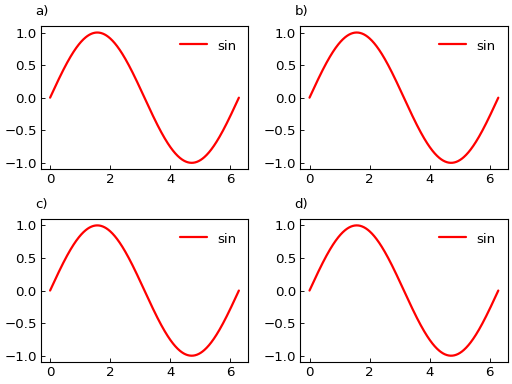
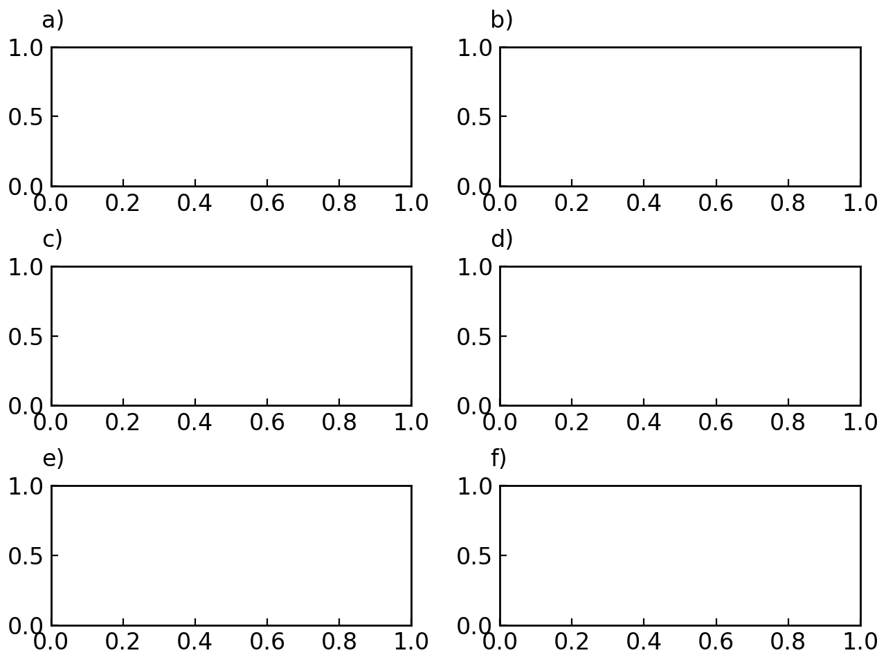
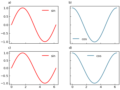
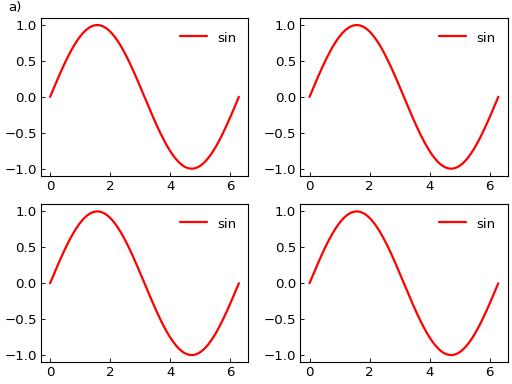
# Disable reference labels
fig = gl.SmartFigure(
    2, 2,
    reference_labels=False,
    elements=[curve1]*4
)
fig.show()

(png, hires.png, pdf)

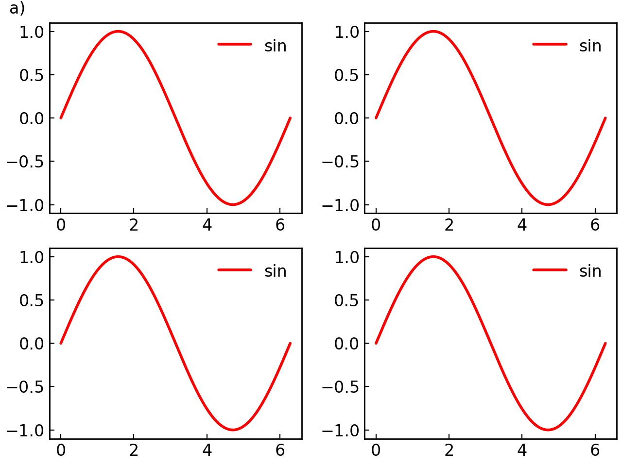
# Show reference labels on specific subplots
fig = gl.SmartFigure(
    2, 2,
    reference_labels=[True, True, False, True],  # No label on third subplot
    elements=[curve1]*4
)
fig.show()

(png, hires.png, pdf)

Reference Label Position

You can control where reference labels are placed using the reference_labels_loc parameter:

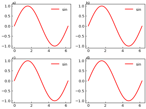
# Inside the plot
fig = gl.SmartFigure(
    2, 2,
    reference_labels_loc="inside",
    elements=[curve1]*4
)
fig.show()

(png, hires.png, pdf)

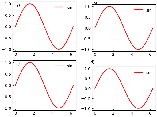
# Custom position (relative to top-left corner)
fig = gl.SmartFigure(
    2, 2,
    reference_labels_loc=(0.02, -0.01),  # (x, y) offset in inches
    elements=[curve1]*4
)
fig.show()

(png, hires.png, pdf)

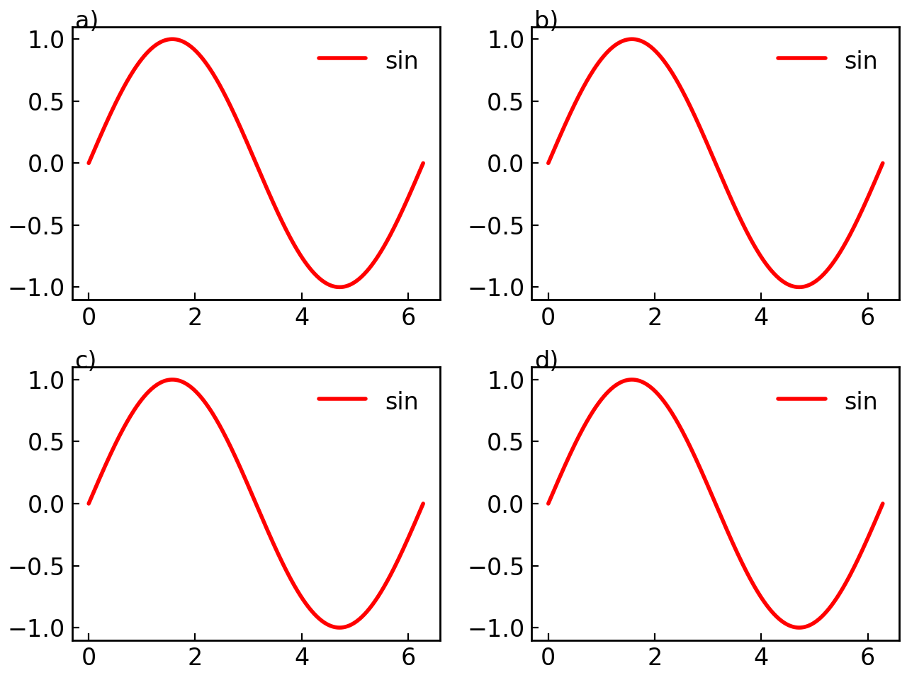
You can also customize the position per subplot:

# Different positions for different subplots
fig = gl.SmartFigure(
    2, 2,
    reference_labels_loc=["inside", (0.05, -0.01), "inside", "outside"],
    elements=[curve1]*4
)
fig.show()

(png, hires.png, pdf)

Global Reference Label

Label the entire figure instead of individual subplots:

fig = gl.SmartFigure(
    2, 2,
    global_reference_label=True,
    reference_labels=False,
    elements=[curve1]*4
)
fig.show()

(png, hires.png, pdf)

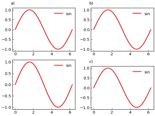
Advanced Reference Label Customization

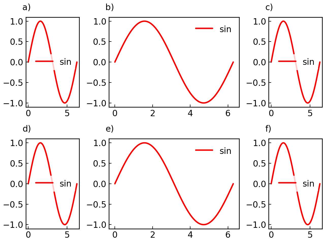
The set_reference_labels_params() method provides detailed control over the reference labels’ appearance:

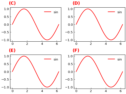
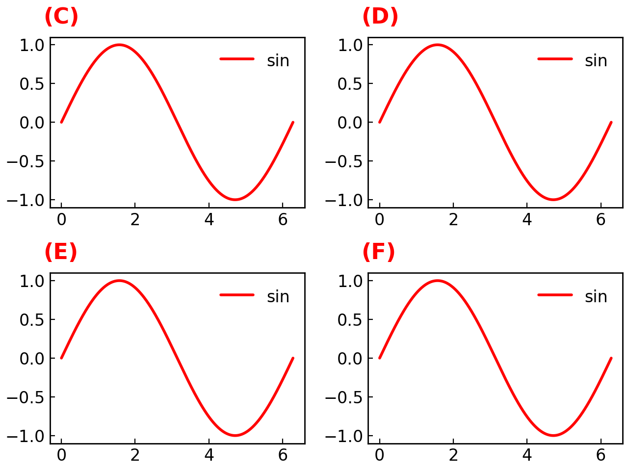
fig = gl.SmartFigure(2, 2, elements=[curve1]*4)

fig.set_reference_labels_params(
    color="red",
    font_size=16,
    font_weight="bold",
    start_index=2,  # Start from "c)"
    format=lambda letter: f"({letter.upper()})"  # (A), (B), etc.
)
fig.show()

(png, hires.png, pdf)

Here we used the format parameter to customize the label format, which can be any function that takes a label letter string as input and returns a formatted string. This function is completely defined by the user, allowing for any desired format.

Note

If you want to have different reference label styles for different subplots, consider using nested SmartFigure objects where each nested figure has its own reference label settings.

Nested SmartFigures

One of the most powerful features is the ability to nest SmartFigure objects within each other.

Basic Nesting

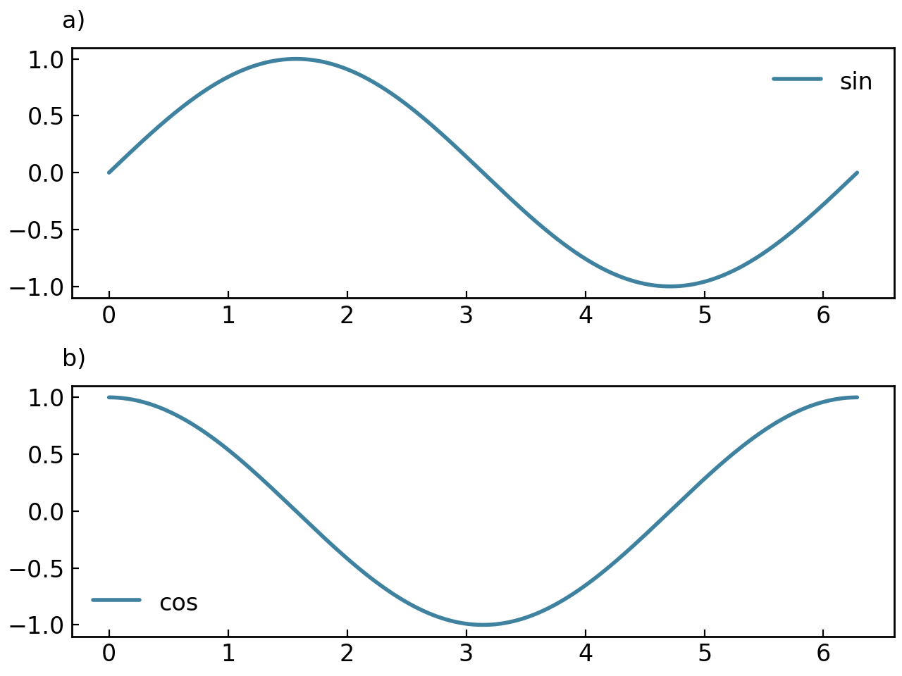
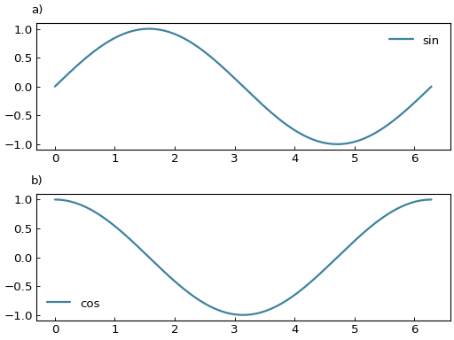
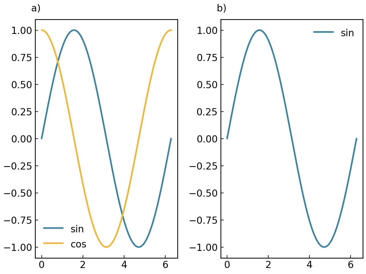
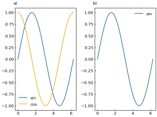
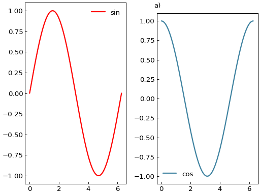
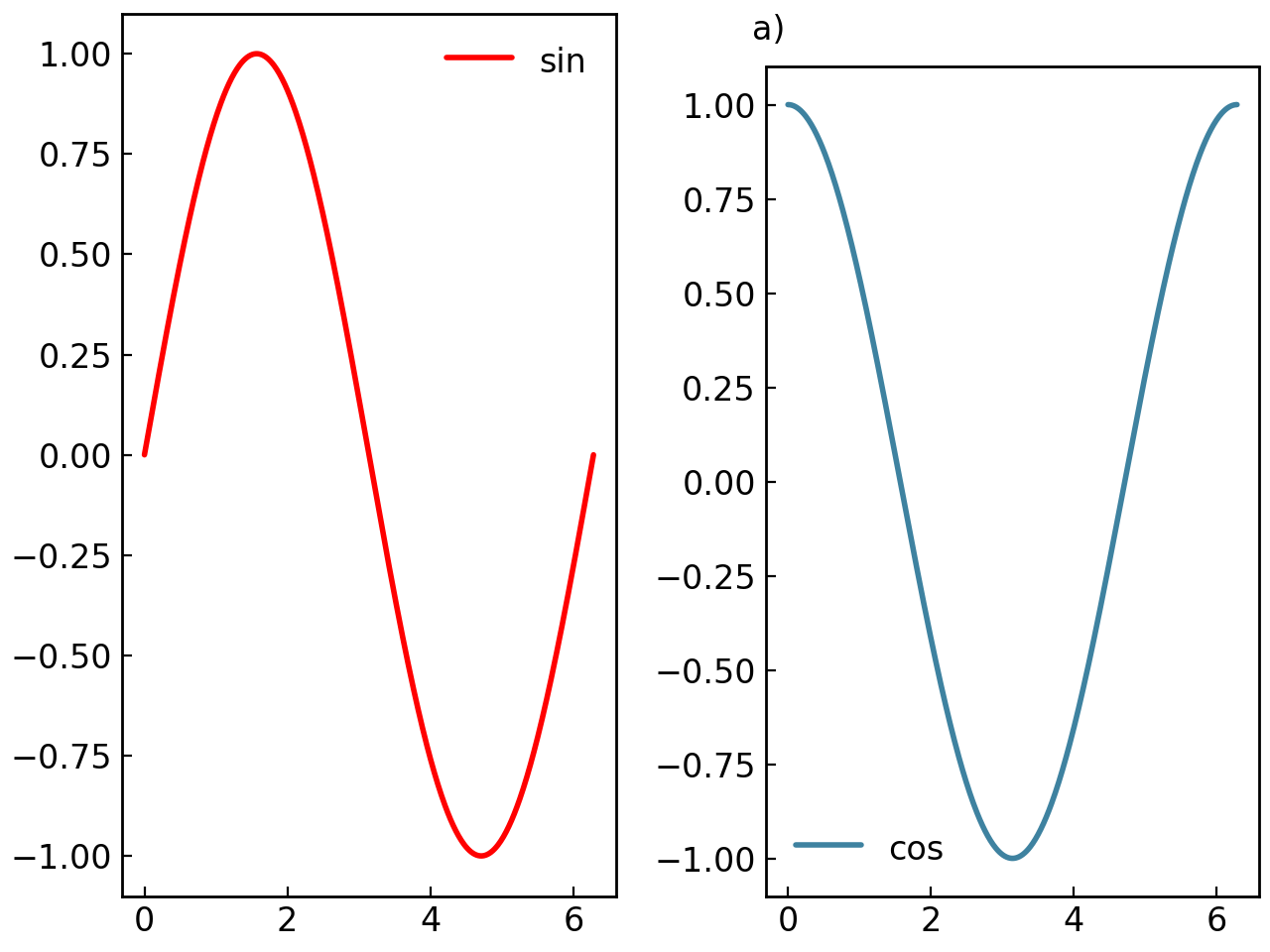
# Create individual figures
fig1 = gl.SmartFigure(elements=curve1, reference_labels=False)
fig2 = gl.SmartFigure(elements=curve2, reference_labels=True)

# Combine them
parent = gl.SmartFigure(num_cols=2, elements=[fig1, fig2])
parent.show()

(png, hires.png, pdf)

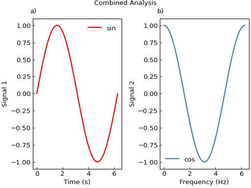
# Each nested figure can have its own parameters
fig1 = gl.SmartFigure(
    x_label="Time (s)",
    y_label="Signal 1",
    elements=curve1,
)
fig2 = gl.SmartFigure(
    x_label="Frequency (Hz)",
    y_label="Signal 2",
    elements=curve2,
)

parent = gl.SmartFigure(
    num_cols=2,
    title="Combined Analysis"
)
parent.elements = [fig1, fig2]
parent.show()

(png, hires.png, pdf)

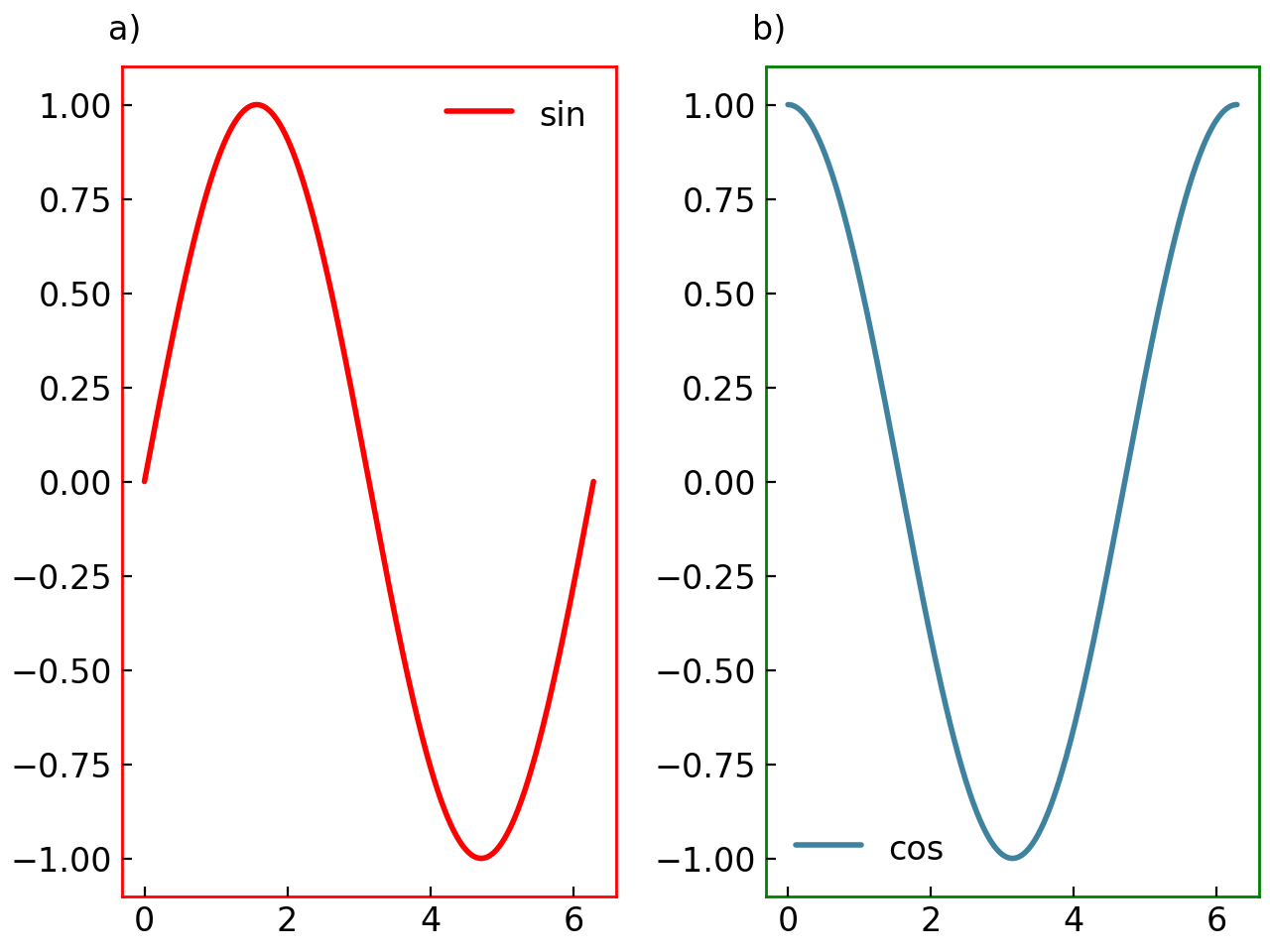
You can also use indexing to modify nested figures after creation:

fig1 = gl.SmartFigure(elements=curve1)
fig2 = gl.SmartFigure(elements=curve2)

parent = gl.SmartFigure(num_cols=2, elements=[fig1, fig2])

# Modify nested figure parameters
parent[0].set_visual_params(axes_edge_color="red")
parent[1].set_visual_params(axes_edge_color="blue")

parent.show()

(png, hires.png, pdf)

Multi-level Nesting

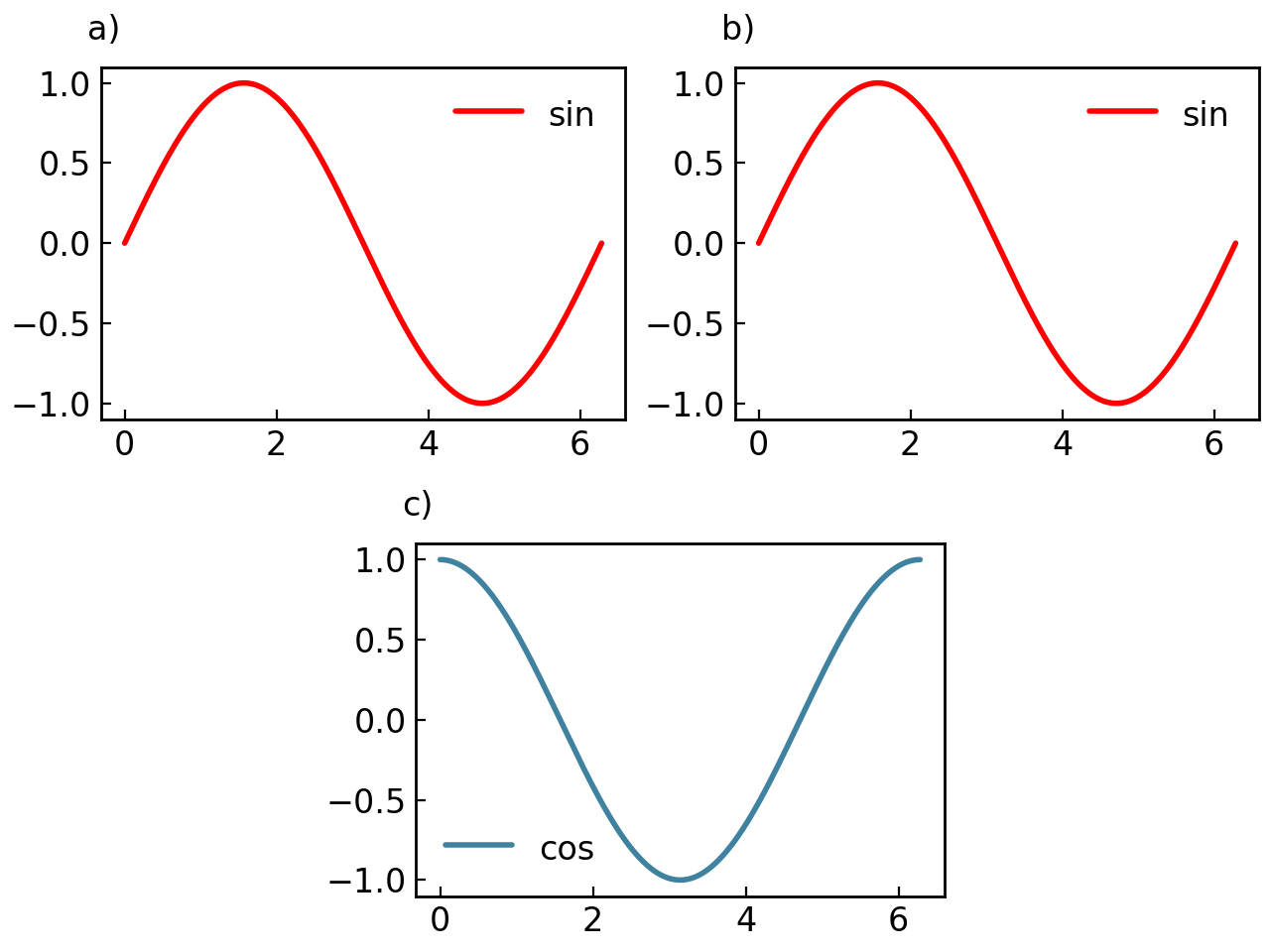
You can nest SmartFigure objects any number of levels deep:

# Level 1: Basic figures
fig_a = gl.SmartFigure(elements=curve1).set_tick_params(color="red", width=10)
fig_b = gl.SmartFigure(elements=curve2).set_tick_params(color="blue", width=10)

# Level 2: Combine into two other figures
row = gl.SmartFigure(num_cols=2, elements=[fig_a, fig_b], global_reference_label=True)
col = gl.SmartFigure(num_rows=2, elements=[fig_a, fig_b], global_reference_label=True)

# Level 3: Combine rows
final = gl.SmartFigure(num_rows=2, num_cols=3)
final[0, :2] = row
final[:, 2] = col
final.show()

(png, hires.png, pdf)

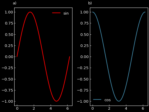
Style Inheritance

The figure_style and visual parameters are inherited by nested figures:

# Parent style applies to all nested figures
fig1 = gl.SmartFigure(elements=curve1)
fig2 = gl.SmartFigure(elements=curve2)

parent = gl.SmartFigure(
    num_cols=2,
    figure_style="dark",  # Applies to fig1 and fig2
    elements=[fig1, fig2]
)
parent.show()

(png, hires.png, pdf)

However, if nested SmartFigure objects specify their visual parameters, those take precedence:

fig1.set_visual_params(axes_edge_color="red")

parent = gl.SmartFigure(num_cols=2, elements=[fig1, fig2])
parent.set_visual_params(axes_edge_color="green")  # fig1 stays red
parent.show()

(png, hires.png, pdf)

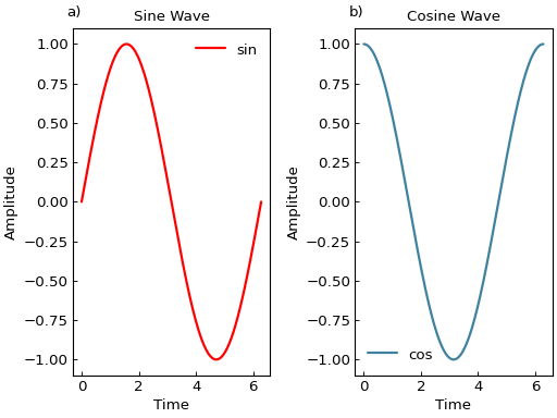
Working with Nested Figures

The copy_with() method is especially useful when working with nested figures:

base_fig = gl.SmartFigure(
    x_label="Time",
    y_label="Amplitude",
    elements=curve1
)

# Create variations
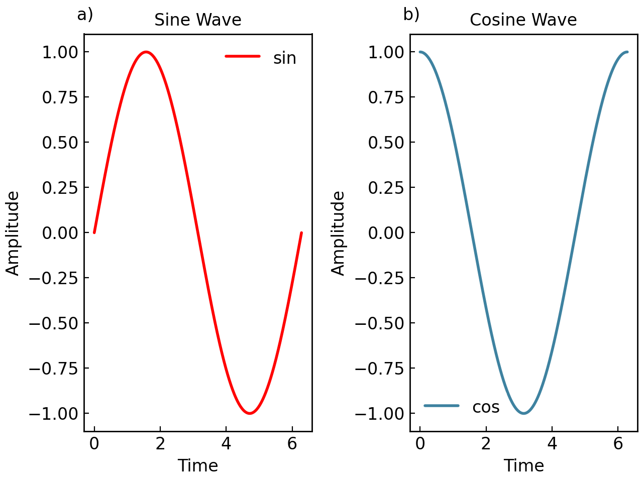
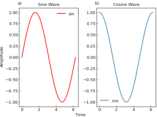
fig1 = base_fig.copy_with(title="Sine Wave")
fig2 = base_fig.copy_with(title="Cosine Wave", elements=curve2)

parent = gl.SmartFigure(num_cols=2, elements=[fig1, fig2])
parent.show()

(png, hires.png, pdf)

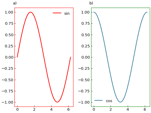
It can also be used to combine figures into a parent figure by changing seamlessly their parameters:

parent = gl.SmartFigure(
    num_cols=2,
    x_label="Time",
    y_label="Amplitude",
    elements=[
        fig1.copy_with(x_label=None, y_label=None),
        fig2.copy_with(x_label=None, y_label=None)
    ]
)
parent.show()

(png, hires.png, pdf)

Twin Axes

The SmartTwinAxis class is very similar to SmartFigure but represents a single secondary axis. This object needs to be associated with a SmartFigure to be displayed and allows you to plot data with different scales on the same subplot. Similar to the SmartFigure you can customize its appearance with set_visual_params(), set_tick_params(), etc. and manage its elements with add_elements() and other methods. For more details, see the SmartTwinAxis class documentation.

Creating Twin Axes

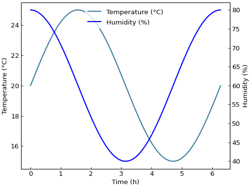
# Create main figure with one curve
temp_curve = gl.Curve.from_function(lambda x: 20 + 5*np.sin(x),
                                    0, 2*np.pi, label="Temperature (°C)")
fig = gl.SmartFigure(
    x_label="Time (h)",
    y_label="Temperature (°C)",
    elements=temp_curve,
)

# Add twin y-axis for humidity data
humidity_curve = gl.Curve.from_function(lambda x: 60 + 20*np.cos(x), 0, 2*np.pi,
                                        label="Humidity (%)", color="blue")

twin_y = fig.create_twin_axis(
    is_y=True,
    label="Humidity (%)",
    elements=humidity_curve,
)

fig.show()

(png, hires.png, pdf)

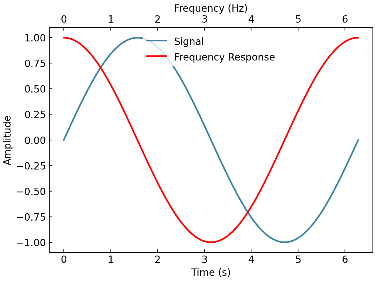
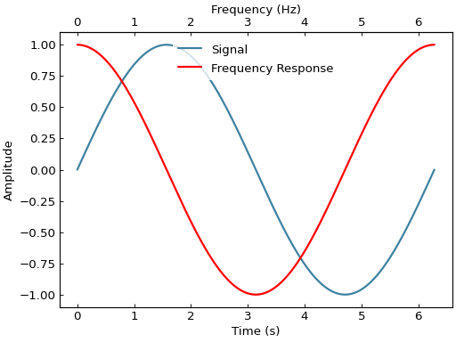
# Twin x-axis
time_curve = gl.Curve.from_function(lambda x: np.sin(x), 0, 2*np.pi, label="Signal")
fig = gl.SmartFigure(
    x_label="Time (s)",
    y_label="Amplitude",
    elements=time_curve,
)

freq_curve = gl.Curve.from_function(lambda x: np.cos(x), 0, 2*np.pi,
                                    label="Frequency Response", color="red")

twin_x = fig.create_twin_axis(
    is_y=False,
    label="Frequency (Hz)",
    elements=freq_curve,
)

fig.show()

(png, hires.png, pdf)

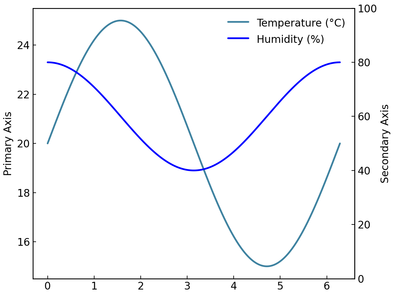
Direct Twin Axis Assignment

Even if the SmartTwinAxis can not be plotted alone, you can create it directly and assign it afterwards to a SmartFigure:

# Create twin axis directly
twin = gl.SmartTwinAxis(
    label="Secondary Axis",
    axis_lim=(0, 100),
    log_scale=False,
    elements=humidity_curve,
)

fig = gl.SmartFigure(
    y_label="Primary Axis",
    twin_y_axis=twin,
    elements=temp_curve,
)
fig.show()

(png, hires.png, pdf)

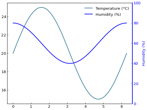
Twin Axis Customization

fig = gl.SmartFigure(elements=temp_curve)

twin_y = fig.create_twin_axis(
    is_y=True,
    label="Humidity (%)",
    axis_lim=(0, 100),
    elements=humidity_curve,
)

# Customize twin axis appearance
twin_y.set_visual_params(
    edge_color="blue",
    label_color="blue",
    line_width=2
)

# Customize twin axis ticks
twin_y.set_tick_params(
    which="major",
    color="blue",
    label_color="blue"
)

fig.show()

(png, hires.png, pdf)

fig = gl.SmartFigure(elements=temp_curve)

# Managing twin axis elements
twin_y = fig.create_twin_axis(is_y=True, elements=humidity_curve)

# Add more elements
extra_curve = gl.Curve.from_function(lambda x: 50 + 10*np.sin(2*x), 0, 2*np.pi,
                                     label="Extra", color="green")
twin_y.add_elements(extra_curve)

# Access elements
first_element = twin_y[0]
print(f"Twin axis has {len(twin_y)} elements")

Output:

Twin axis has 2 elements

Note

Twin axes can only be created for single-subplot SmartFigure objects (1x1 grid). As such, it may be required to use nested SmartFigure objects when working with multi-subplot figures that need twin axes.

Projections

The SmartFigure supports various coordinate system projections through the projection parameter. This allows you to display data in non-Cartesian coordinate systems such as polar coordinates or astronomical World Coordinate Systems (WCS).

Supported Projections

The projection parameter accepts:

• Matplotlib projection strings: Any projection name supported by matplotlib (e.g., "polar", "aitoff", "hammer", "lambert", "mollweide", "rectilinear"). You can get a list of available projections using matplotlib.projections.get_projection_names().

• Projection objects: Objects capable of creating a projection. For astropy.wcs.WCS objects used for plotting astronomical data, use the specialized SmartFigureWCS class instead. You can read more about it in the Specialized SmartFigures for different projections documentation. Install the graphinglib[astro] extra to enable WCS support.

Warning

3D projections ("3d") are not supported at this time. These will be added in a future release, probably as a separate class SmartFigure3D.

Basic Projection Usage

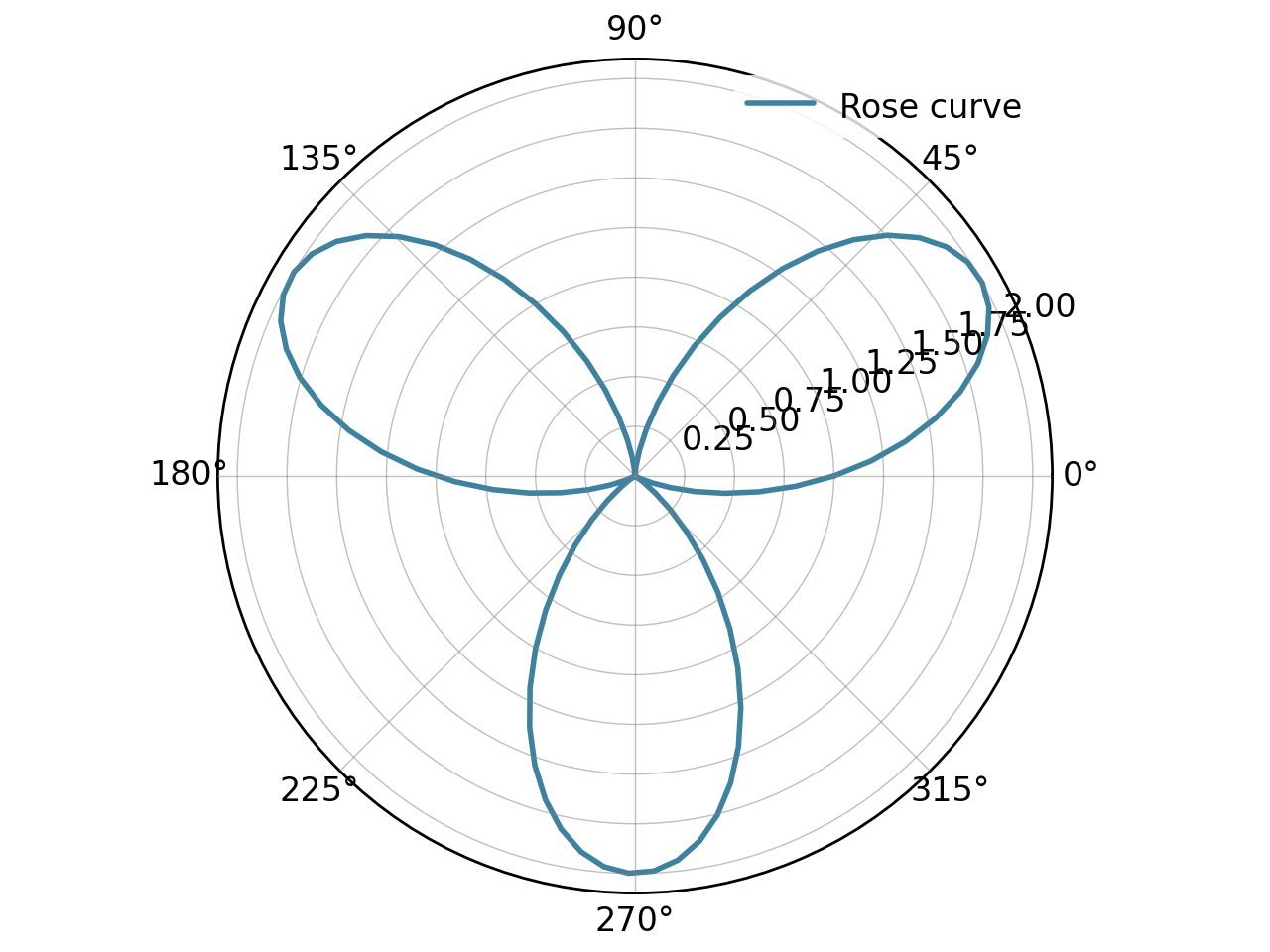
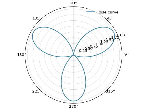
Polar Projection

The most common projection is the polar coordinate system:

# Create data in polar coordinates
theta = np.linspace(0, 2*np.pi, 100)
r = 1 + np.sin(3*theta)

# Create curve using polar projection
polar_curve = gl.Curve(theta, r, label="Rose curve")

fig = gl.SmartFigure(
    projection="polar",
    aspect_ratio="equal",
    elements=polar_curve,
)
fig.show()

(png, hires.png, pdf)

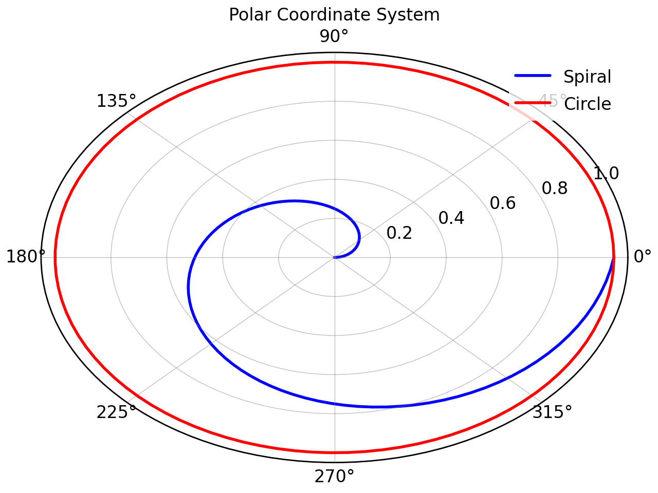
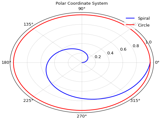
# Multiple elements in polar coordinates
spiral = gl.Curve(
    theta,
    theta / (2*np.pi),
    label="Spiral",
    color="blue"
)
circle = gl.Curve(
    theta,
    np.ones_like(theta),
    label="Circle",
    color="red"
)

fig = gl.SmartFigure(
    projection="polar",
    title="Polar Coordinate System",
    elements=[spiral, circle]
)
fig.show()

(png, hires.png, pdf)

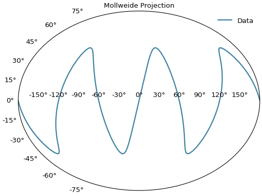
Other Matplotlib Projections

Matplotlib provides several map-like projections useful for displaying data on spherical surfaces:

# Mollweide projection (useful for world maps)
lon = np.linspace(-np.pi, np.pi, 100)
lat = np.sin(3*lon) * np.pi/4

curve = gl.Curve(lon, lat, label="Data")

fig = gl.SmartFigure(
    projection="mollweide",
    title="Mollweide Projection",
    elements=curve,
)
fig.show()

(png, hires.png, pdf)

See also

See the Matplotlib Projections Documentation for more details on available projections and their usage.

Projections with Multiple Subplots

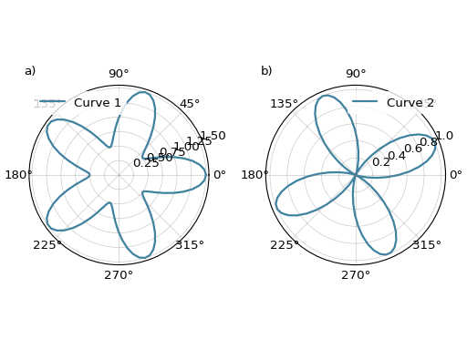
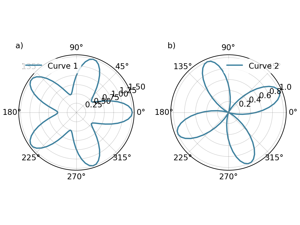
When using projections with multi-subplot figures, all subplots share the same projection:

# All subplots will use polar projection
theta = np.linspace(0, 2*np.pi, 100)
r1 = 1 + 0.5*np.cos(5*theta)
r2 = 0.5 + 0.5*np.sin(4*theta)

curve1 = gl.Curve(theta, r1, label="Curve 1")
curve2 = gl.Curve(theta, r2, label="Curve 2")

fig = gl.SmartFigure(
    1, 2,
    aspect_ratio="equal",
    projection="polar",
    elements=[curve1, curve2]
)
fig.show()

(png, hires.png, pdf)

Note

If you need different projections for different subplots, use nested SmartFigure objects where each can have its own projection.

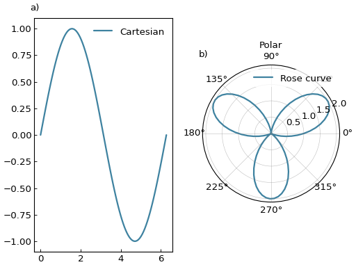
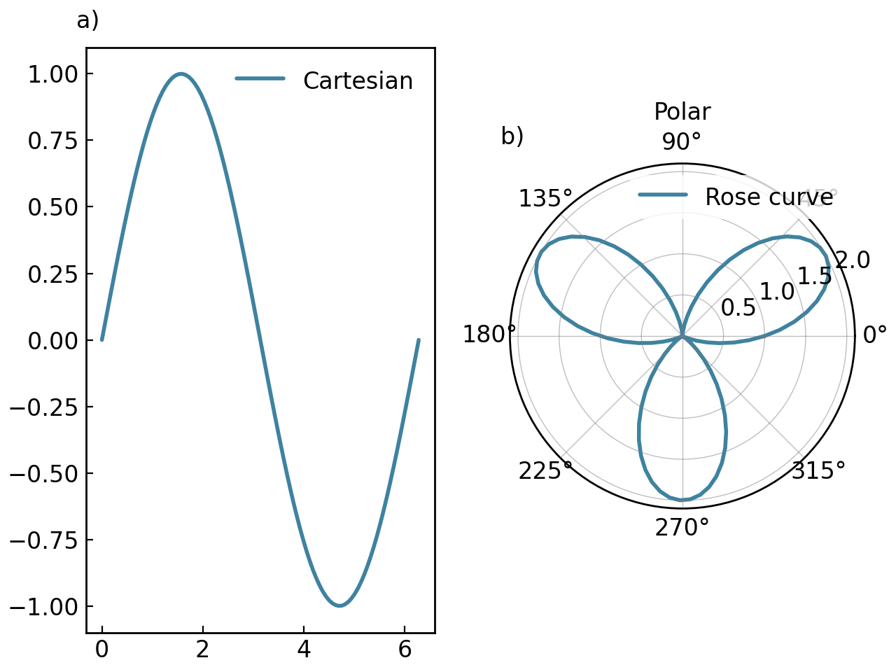
Projections with Nested Figures

Nested figures can have different projections:

# Create a Cartesian curve
x = np.linspace(0, 2*np.pi, 100)
y = np.sin(x)
cartesian_curve = gl.Curve(x, y, label="Cartesian")

# Create a polar figure
polar_fig = gl.SmartFigure(
    projection="polar",
    aspect_ratio="equal",
    title="Polar",
    elements=polar_curve,
)

# Combine them
parent = gl.SmartFigure(
    num_cols=2,
    elements=[cartesian_curve, polar_fig]
)
parent.show()

(png, hires.png, pdf)

Astronomical Data with SmartFigureWCS

For plotting astronomical data with World Coordinate System (WCS) projections, GraphingLib provides the specialized SmartFigureWCS class. This class extends SmartFigure with features specifically designed for astronomical coordinate systems.

Key features of SmartFigureWCS:

• Automatic celestial coordinate formatting (RA/Dec, Galactic, etc.)

• Support for FITS WCS metadata

• Curved coordinate grid lines following great circles

• All standard SmartFigure features (nesting, twin axes, styling, etc.)

See also

See Specialized SmartFigures for different projections for comprehensive documentation on plotting astronomical data with SmartFigureWCS.

File Operations

Displaying Figures

The show() method displays a SmartFigure:

fig = gl.SmartFigure(elements=curve1)

# Basic display
fig.show()

# Fullscreen display
fig.show(fullscreen=True)

Warning

For figures with general legends in “outside” positions, use inline Jupyter display or save to a file for correct rendering.

Saving Figures

The save() method is used to save the figure to various formats:

fig = gl.SmartFigure(elements=curve1)

# Save as PNG
fig.save("output.png", dpi=300)

# Save as PDF
fig.save("output.pdf")

# Save with transparent background
fig.save("output.png", transparent=True)

Split PDF Saving

The split_pdf parameter allows the SmartFigure to save each of its subplot on a separate PDF page:

fig = gl.SmartFigure(2, 2, elements=[curve1]*4)

# Each subplot becomes a separate page
fig.save("multi_page.pdf", split_pdf=True)

If you want however to save multiple SmartFigure objects into a single multi-page PDF, you can use PdfPages from matplotlib.backends.backend_pdf:

from matplotlib.backends.backend_pdf import PdfPages

with PdfPages("output.pdf") as pdf:
    fig1.save(pdf)
    fig2.save(pdf)
    fig3.save(pdf)

Utility Methods and Properties

Copying Figures

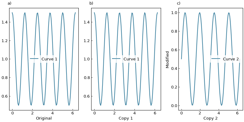
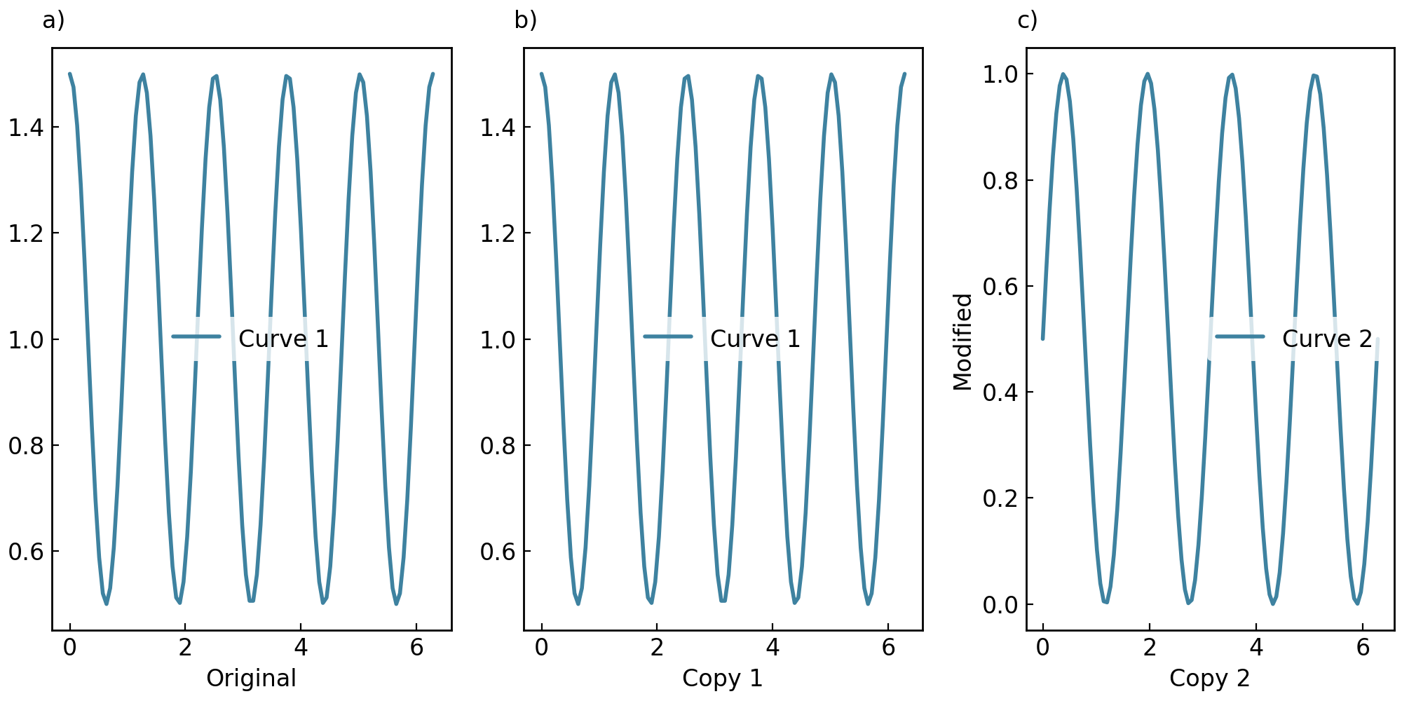
Both copy() and copy_with() methods create copies of a SmartFigure. The former creates a deep copy, while the latter also deep copies but allows you to modify specific parameters at the same time:

original = gl.SmartFigure(
    x_label="Original",
    elements=curve1,
)

# Deep copy
copy1 = original.copy()
copy1.x_label = "Copy 1"

# Copy with modifications
copy2 = original.copy_with(
    x_label="Copy 2",
    y_label="Modified",
    elements=curve2,
)

parent = gl.SmartFigure(num_cols=3, size=(10, 5), elements=[original, copy1, copy2])
parent.show()

(png, hires.png, pdf)

Inspecting Figures

fig = gl.SmartFigure(2, 3, elements=[curve1]*6)

# Get number of child plots in the layout
print(f"Number of child plots: {len(fig)}")  # 6

# Get shape
print(f"Shape: {fig.shape}")  # (2, 3)

# Check if the figure is currently used as a single plot
print(f"Is single subplot: {fig.is_single_subplot}")  # False

single_fig = gl.SmartFigure(elements=curve1)
print(f"Is single subplot: {single_fig.is_single_subplot}")  # True

# Access a specific child plot
child_plot = fig[0, 0]
print(f"Elements in (0,0): {len(child_plot.elements)}")

Method Chaining

Most methods return self to enable method chaining:

fig = (gl.SmartFigure(elements=curve1)
       .set_visual_params(axes_edge_color="red")
       .set_ticks(x_tick_spacing=1.0)
       .set_tick_params(direction="out")
       .set_grid(color="gray", alpha=0.3))

fig.show()

(png, hires.png, pdf)

Complete Configuration Example

Here’s a comprehensive example using many advanced features:

# Create base data
x = np.linspace(0, 2*np.pi, 100)
y1 = np.sin(x)
y2 = np.cos(x)
y3 = np.sin(2*x)
y4 = np.cos(2*x)

# Create curves
curve1 = gl.Curve(x, y1, label="sin(x)", color="blue")
curve2 = gl.Curve(x, y2, label="cos(x)", color="red")
curve3 = gl.Curve(x, y3, label="sin(2x)", color="green")
curve4 = gl.Curve(x, y4, label="cos(2x)", color="orange")

# Create nested figures
fig_top_left = gl.SmartFigure(
    title="Fundamental Frequencies",
    elements=[curve1, curve2]
)

fig_top_right = gl.SmartFigure(
    title="Harmonics",
    elements=[curve3, curve4]
)

# Create bottom spanning figure
fig_bottom = gl.SmartFigure(
    title="Combined View",
    elements=[curve1, curve2, curve3, curve4]
).set_visual_params(
    axes_edge_color="purple",
    hidden_spines=["top", "right"]
)
fig_bottom.hide_default_legend_elements = True  # prevent duplicate legend entries

# Combine into parent figure
parent = gl.SmartFigure(
    num_rows=2,
    num_cols=2,
    size=(10, 6),
    figure_style="plain",
    title="Comprehensive Signal Analysis",
    general_legend=True,
    legend_loc=(0.3, 0.46),
    legend_cols=4,
    width_padding=0.02,
    height_padding=0.07
)

# Add elements with spanning
parent.elements = [fig_top_left, fig_top_right]
parent[1, :] = fig_bottom  # Spans both columns

# Global customization
parent.set_visual_params(
    figure_face_color="#c7c4c4",
    font_size=11,
    title_font_size=14,
    title_font_weight="bold"
)

# Add global annotation
note = gl.Text(1, 1, "Generated with GraphingLib",
            h_align="right",
            v_align="top",
            font_size=8,
            color="gray")
parent.annotations = [note]

parent.show()

(png, hires.png, pdf)

Best Practices and Tips

Element Management

1. Use the right method for the job:

   • Use __init__ or elements property for initial setup

   • Use add_elements() for incremental additions

   • Use __setitem__ (indexing) for spanning elements or precise control

2. Understand None behavior:

   • None → subplot not drawn (blank space)

   • [None] or [] → subplot drawn but empty

   • Useful for creating asymmetric layouts

3. Element removal:

   • Use exact slice for removing spanning elements

   • fig[row, col] = None only removes elements at that exact position

Layout Design

1. Use copy_with() for variations:

   Create a base figure and make copies with modifications instead of recreating from scratch.

2. Plan your grid:

   Sketch your layout before coding. Use width_ratios and height_ratios for non-uniform sizes.

3. Leverage nesting:

   Break complex figures into smaller SmartFigure objects and combine them.

Styling

1. Start with a style file:

   Define your base appearance in a style file, then customize specific figures.

2. Layer your customizations:

   • Figure style (broadest)

   • set_visual_params() or set_rc_params() (figure-specific)

   • Individual element properties (finest control)

3. Nested figure styling:

   Remember that parent figure_style applies to all children, but child customizations override parent customizations.

Legends

1. Choose legend type wisely:

   • Individual legends: Simple figures, different data types per subplot

   • General legend: Related data across subplots, cleaner appearance

2. Custom legend elements:

   Use for theoretical lines, annotations, or elements not directly plotted.

3. Control visibility:

   Use hide_default_legend_elements and hide_custom_legend_elements for precise control.

Troubleshooting

Figure too crowded:

Increase width_padding/height_padding or adjust size.

Labels overlapping:

Use set_text_padding_params() to add spacing. You can even set negative padding values to reduce space.

Subplots slightly misaligned:

If suplots in the same row/column are not perfectly aligned, make sure that no tick label is overlapping into the margins between subplots, as this causes matplotlib to force different subplot sizes to fit the tick label in the available box.

Can’t remove spanning element:

Ensure you’re using the exact slice used to add it.

Legend not showing:

Verify that the elements have labels, that show_legend=True, and that hide_default_legend_elements or hide_custom_legend_elements are False.

Grid not visible:

Call set_grid() first, then verify that show_grid is True.

Twin axis error:

Verify figure is single-subplot (is_single_subplot == True). You may need to create a nested SmartFigure for the subplot with twin axis.

GraphingLib issues:

GraphingLib/GraphingLib#issues

See Also

• Creating a simple figure with the SmartFigure - Quick start guide

• Specialized SmartFigures for different projections - Plotting astronomical data with WCS

• Writing your own figure style file - Creating custom style files

• graphinglib.SmartFigure - SmartFigure API reference

• graphinglib.SmartTwinAxis - Twin axis API reference

• graphinglib.SmartFigureWCS - WCS figure API reference

• Matplotlib projections - Available projection types